Ernst Siemens was first person to design a moving coil transducer. After registering a German patent for the device, he received a U.S. patent in 1874. Inventors and engineers continued to refine the concept over the next 100 or more years. Figure 4.1 shows the components of a modern moving coil loudspeaker. The device is also referred to as an electro-dynamic speaker.
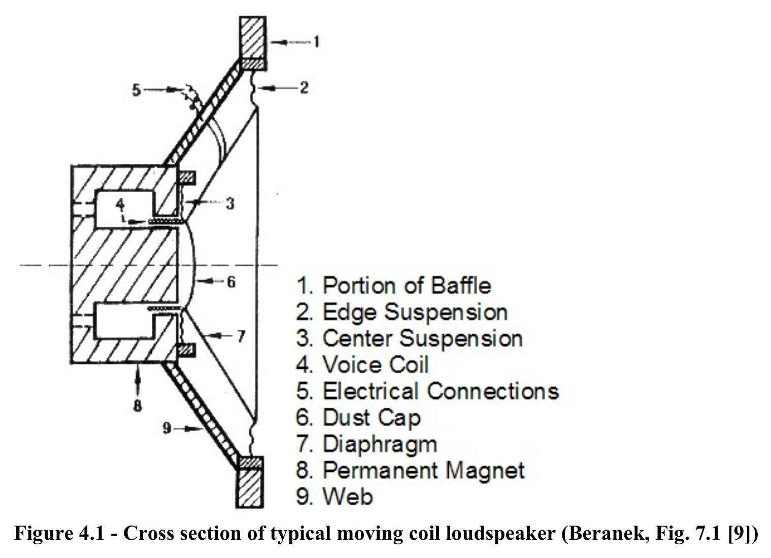
To model the system, include this device as the transducer in the conceptual model of an acoustic transmitter shown in Figure 3.2. A simple way to include the amplifier that supplies power to the electrical connections (item 5 in Figure 4.1) is needed. The amplifier can be considered an effort (voltage) source,
can be considered an effort (voltage) source,
in series a resistance Rg. The current flows through the voice coil (item 4 in Figure 4.1) that is suspended in a magnetic field. The voice coil has both inductance LE and resistance RE. The coil in a magnetic field with oscillating current acts as a gyrator causing a force on the diaphragm. The moving coil generates a back emf,
The moving coil generates a back emf,
in the electrical
circuit. Figure 4.2 shows the electrical circuit. Figure 4.3 shows a bond graph tile for this part of the device, plus it explicitly shows the signal source, element AB100, that modulates the amplifier voltage.
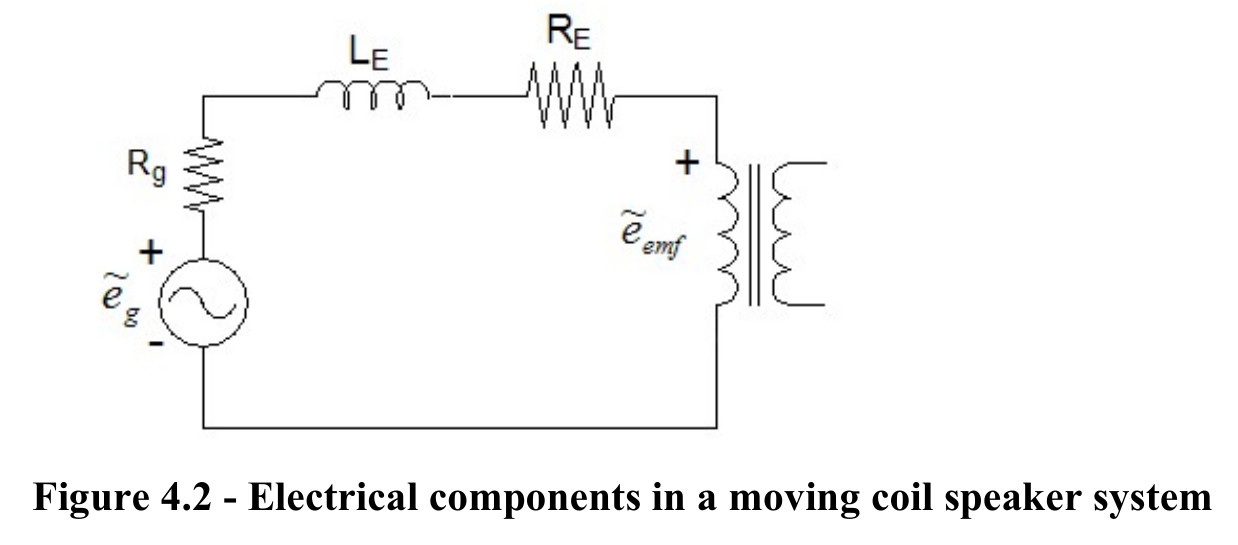
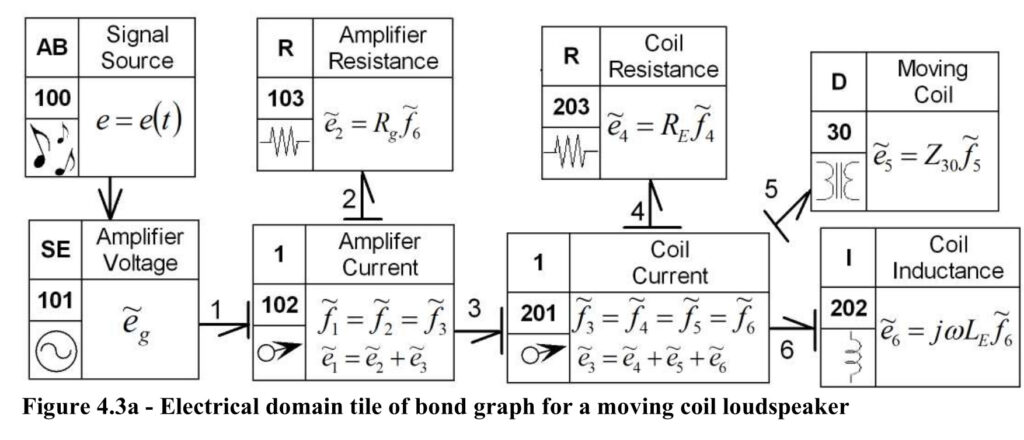
Figure 4.3a has two 1-junctions connected to each other. Separating the amplifier current from the coil current has advantages if there will be a need to model the amplifier in more detail, or if line characteristics will be added between the amplifier and the driver, but for this discussion the model can be simplified by merging the two 1-junctions to give Figure 4.3b. Figure 4.3b is further simplified by implicitly including AB100 in SE101, and using causality to remove unnecessary variables.
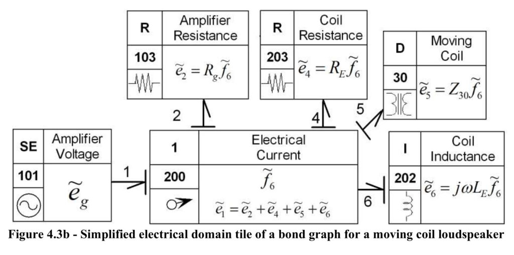
Current flow is the causal variable entering the moving coil, D30. Lorentz’s Law is used to describe its behavior.

and since power is conserved through a gyrator

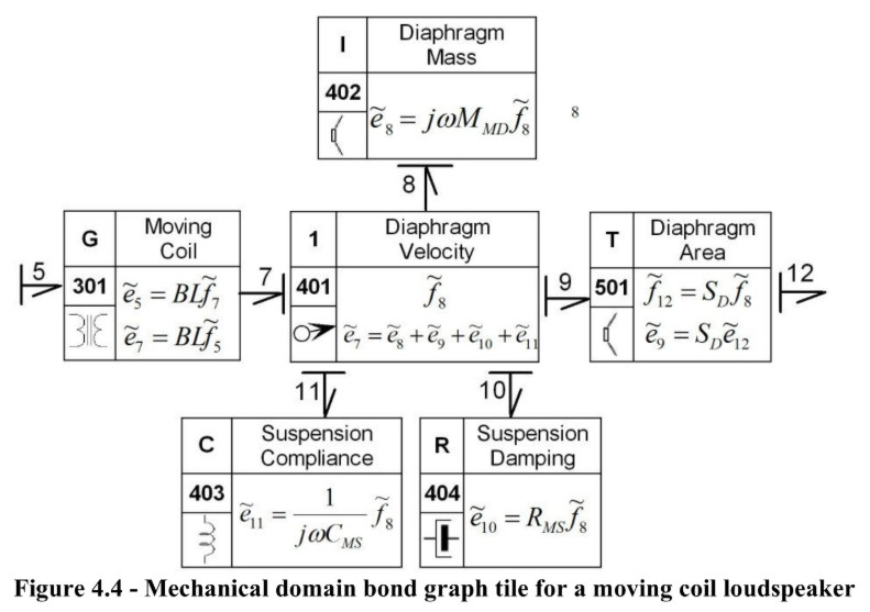
The mechanical part of the speaker is next. The moving coil, the diaphragm, and the suspension all move together to drive the air that is in contact with the diaphragm. All the moving mass can be lumped into MMD. Similarly both the edge suspension compliance and the center suspension compliance are lumped into CMS, and the suspension damping is characterized by RMS. Figure 4.4 shows a bond graph tile for the mechanical part of the speaker. The diaphragm area, SD, is the transformer modulus of T501, that
convertst the diaphragm velocity,
into the volume velocity,
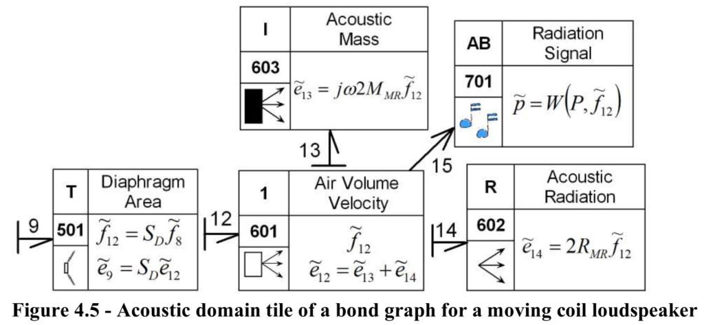
To finish the model, the constitutive equation for the acoustic pressure on the speaker diaphragm is needed. Following the approach discussed in Chapter 3, a complex impedance, ZA is used with

Equation {4.3} has the factor 2 because the speaker diaphragm has 2 sides (assumed to be identical) that move air.
Equation {4.3} is put into an accession to inertia form by letting

Figure 4.5 shows the bond graph tile for the acoustic domain.
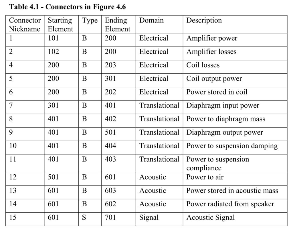
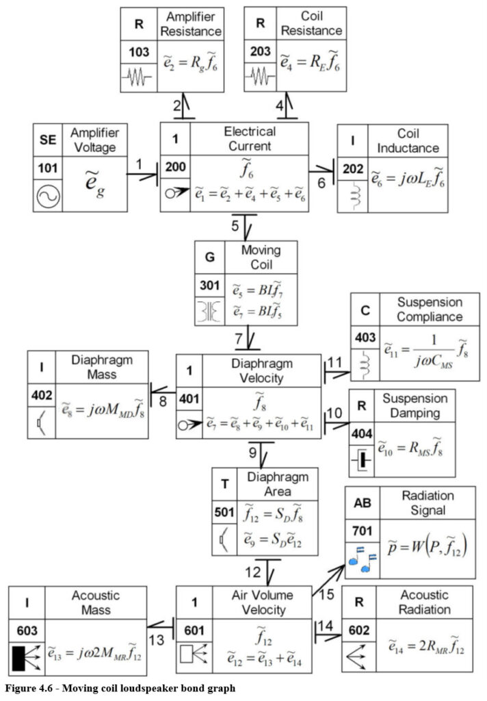
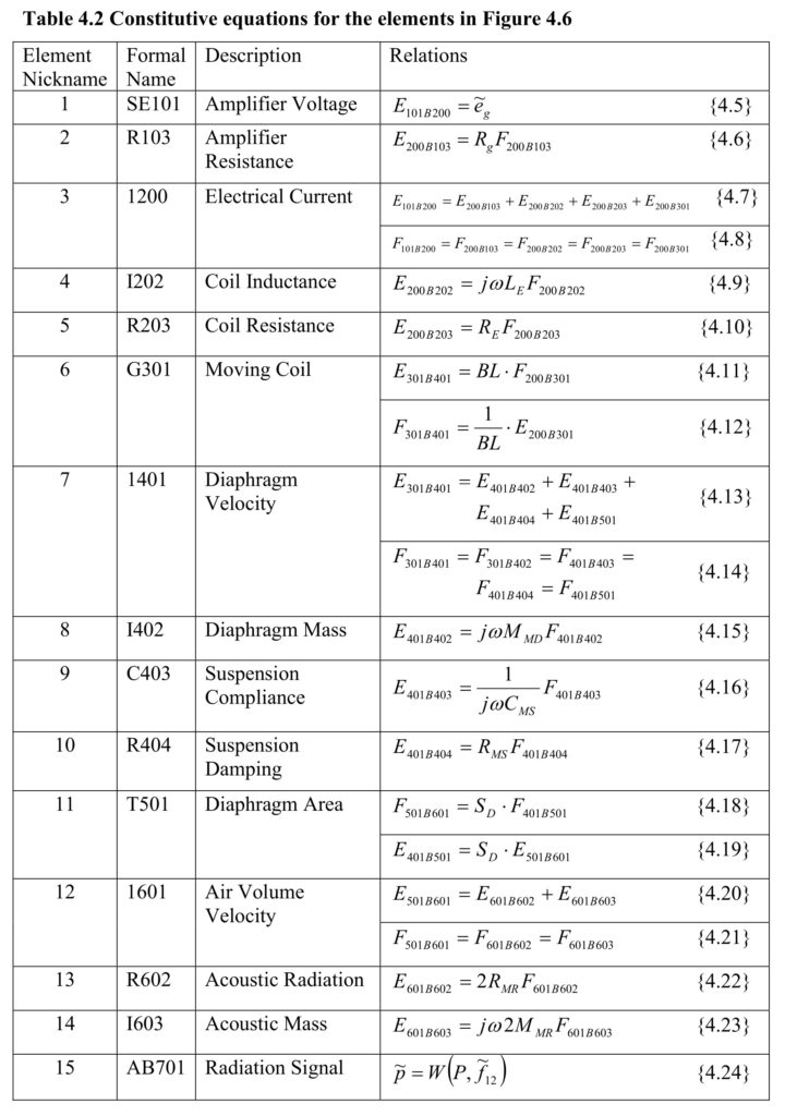
Figures 4.3b, 4.4, and 4.5 are combined to complete the bond graph in Figure 4.6. The bond graph in Figure 4.6 can be summarized by describing the connectors in Table 4.1, and the elements in Table 4.2.
Radiated Power
The acoustic power radiated by a loudspeaker is an important system characteristic. Recall from Equation {2.66} that

is the power radiated from an acoustic resistance. This quantity is calculated from the power flowing to element R602 as a function of the Amplifier Voltage specified by SE101.

Since RMR is a real number, the constitutive equation, {4.22}, cannot induce a phase shift between E601B602 and F601B602. Since the phase angle between the effort and flow is zero,

The set of equations in Table 4.2 can be solved to get F601B602 in terms of the input voltage Eg. Figure 4.7 shows how Figure 4.6 can be simplified. Step 1 is to use the flow equivalences provided by Elements 200, 401, 601, to reduce the number of flow variables, take most of the one-port elements into the junctions, and ignore any signal processing blocks.
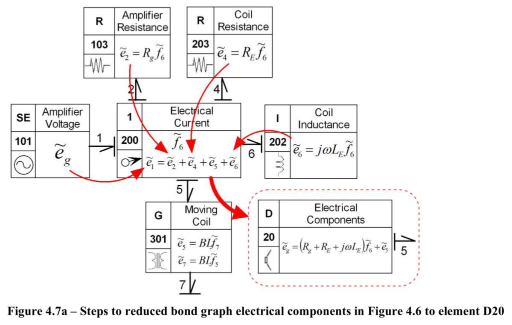
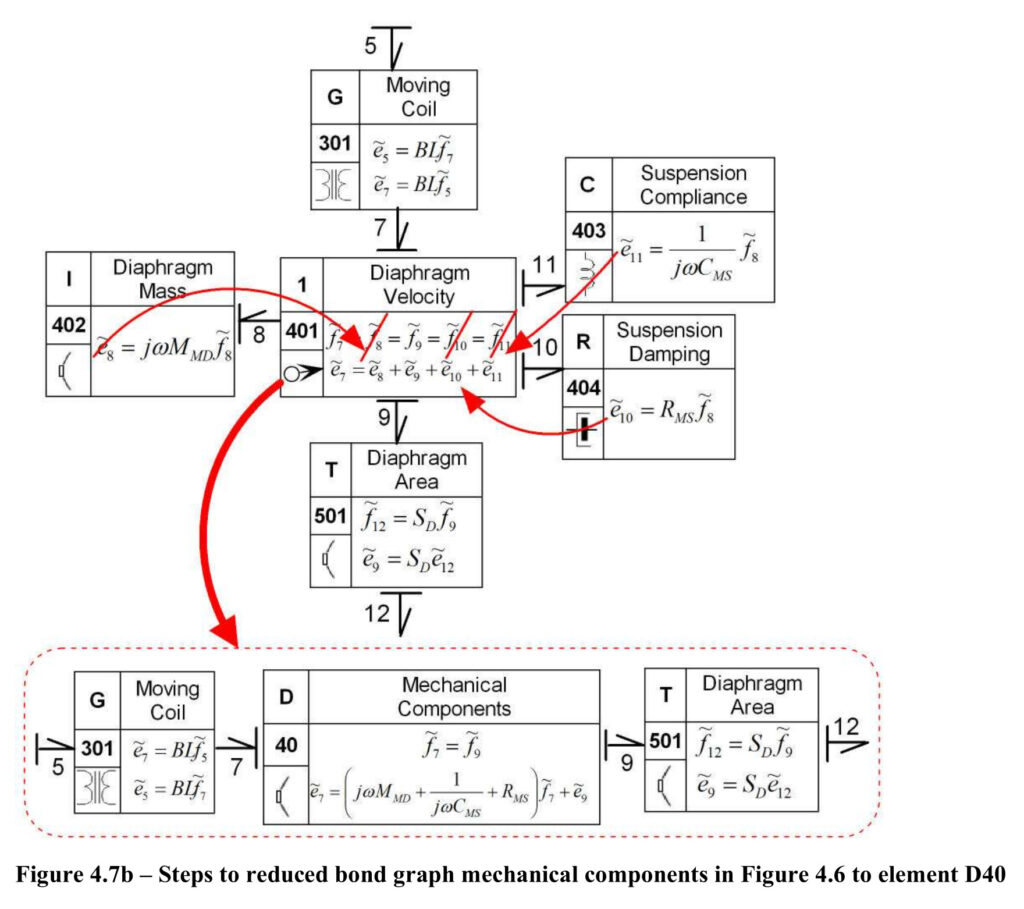
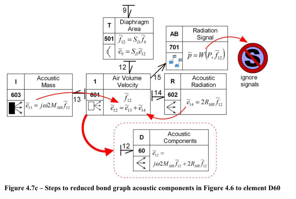
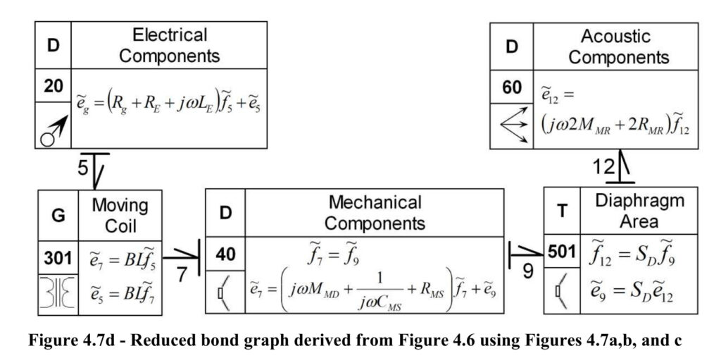
The bond graph in Figure 4.7d can be reduced by moving the gyrator and transformer equations in elements 301 and 501 into their neighbors as shown in Figure 4.8a to give Figure 4.8b.
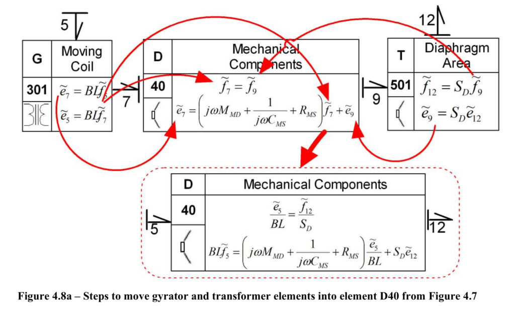
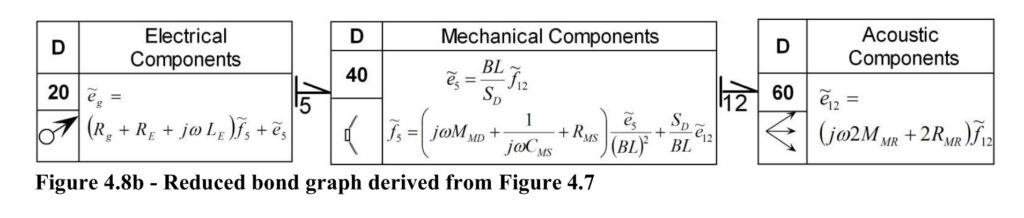
Figure 4.8b is prepared to bring D20 and D60
into D40 by using
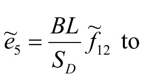
remove
in the bond graph shown in Figure 4.8c
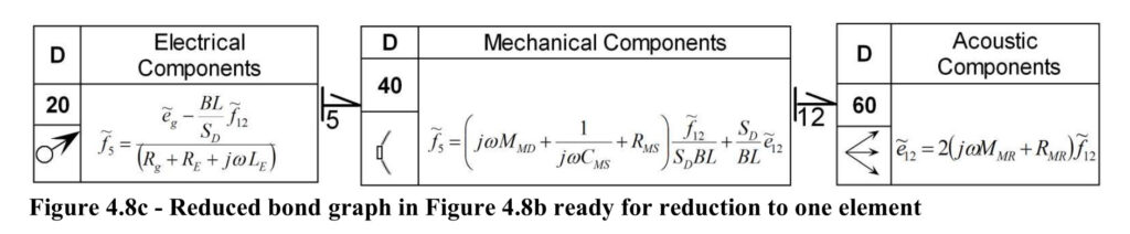
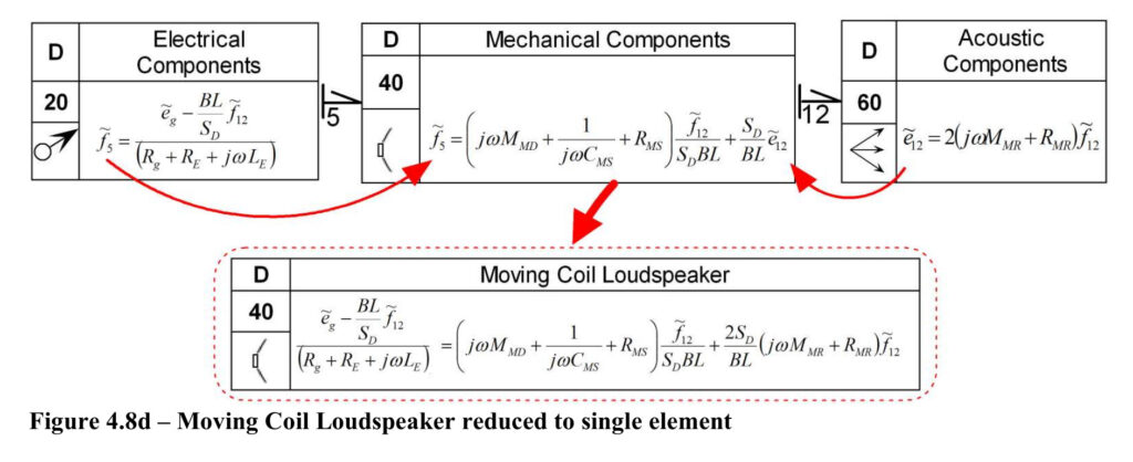
Figure 4.8d shows the final single element bond graph that gives the equation for the acoustic volume velocity amplitude at the face
of the speaker,
as a function of the voltage amplitude,
.
With a little algebra, the equation in D40, can be written in impedance form as

with

The power equation {4.26} needs F601B602 which from {4.27}

Therefore, substituting {4.29} gives

The equation for Z40 can be simplified by making the following substitutions.
Let




Over the frequency range of interest (20 Hz to 20 kHz) the inductance of the coil is small compared to its resistance, therefore

and
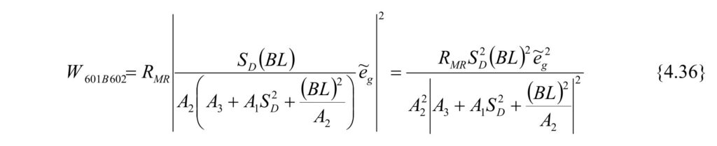
Note, all the terms outside the absolute value signs are not complex numbers.
With

and

Equation {4.36} can be rewritten as

Equation {4.39} can be shown to equal {4.36} using the definition
for the magnitude of a complex number,
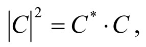
where * indicates complex conjugate.
Relationship between Radiated Pressure and Power
In the previous section, a relationship for the power radiated from a loudspeaker was developed. Now the relationship for sound pressure will be determined.
Average sound intensity, I, is the time average rate of energy flow through a unit area of the medium, or power/area.
As stated in Chapter 3 for a spherical source,

Where
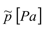
is the peak pressure,
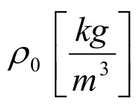
is the medium
density, and
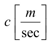
is the speed of sound in the medium.
The term
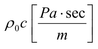
is called the characteristic impedance.
From Chapter 3, intensity for a spherical source with
surface area
is

Combining {4.40} and {4.41} gives the relationship between power and pressure amplitude in the far field for an omnidirectional source:

Solving for the pressure amplitude, {4.42} gives

For a directional radiating source, the pressure amplitude given by{4.43} is scaled by the Directivity Factor, γ as defined in Chapter 3
When a directional source radiates only into a half space, use

for the power, therefore

Solving {4.45} for the magnitude of the pressure amplitude

Then substituting {4.39} into {4.46}

The ratio of the magnitude of pressure amplitude and input voltage for a specified value of r is called the transmitting voltage response, TVR. Thus

Equation {4.48} can be graphed as a function of frequency by using Matlab or some other application to examine the variation of the function with frequency, but by performing order analysis on the equations a feel for the character of the frequency response can be obtained.
Of the variables in {4.48} only 4 parameters are functions of frequency:

For a baffled circular piston radiating into a half space, the directivity factor for the principal axis is given by:

Where k is the wave number, a is the radius of the piston, and J1 is the Bessel Function of Order 1. For the same type of source (baffled circular piston radiating into a half space)

The symbol “~” means “is of order”. Therefore

Although this development was started considering a baffled circular piston, this result is valid for any size or shape baffled piston.
Considering just the frequency characteristics of the TVR, substituting {4.51} into {4.48} gives that the on-axis TVR is proportional to:

The parameter RM given by {4.37} is dominated by the first and second terms thus

which at the level modeled here do not vary with frequency.
The relationship for XM given by {4.38} has three regions defined by the principal resonance frequency, ω0, which occurs when

therefore

At frequencies below ω0, the mechanical impedance of the speaker is stiffness controlled


At the resonance frequency,
the height of the peak
response is damping controlled. One metric for damping is the mechanical quality factor, QM,

Good speaker design practice is to have
Above the principal resonance frequency, the impedance is mass controlled

then

and

At high frequencies, the cone vibration breaks into opposite phase regions with an attendant reduction in radiation efficiency. Also, at high frequency the coil inductance, LE, can no longer be ignored. For these reasons, this analysis is invalid for frequencies more than 1 decade above ω0.
Figure 4.9, is a sketch of the frequency response for a baffled loudspeaker with alternative values for QM.
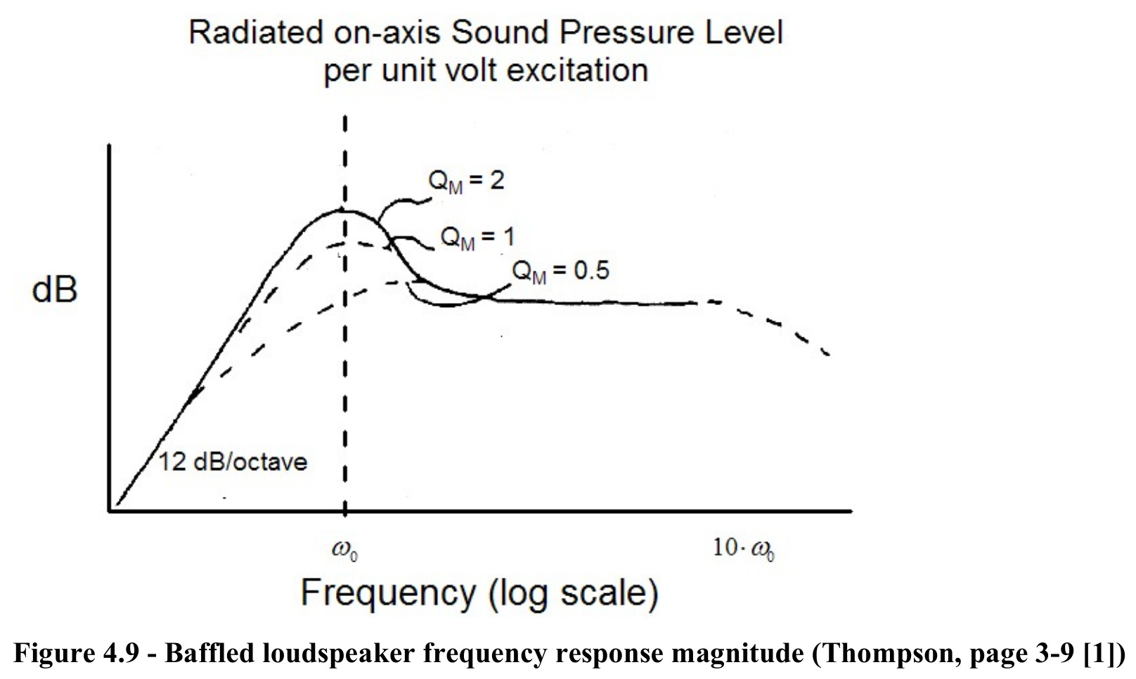
Four frequency response regions are shown in Figure 4.9. At low frequencies, the gain increases with a slope of ω2.
Since
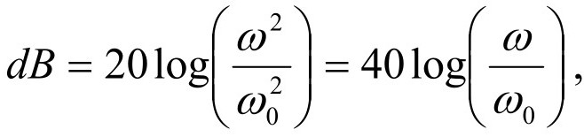
the rise for 1 octave of run is

The slope of the low frequency line is 12 dB/octave.
The region around the resonance frequency has a peak that depends on the value of QM.
At frequencies above the resonance frequency but below the validity limit of the model, the frequency response is flat. This flatness is a reason moving coil loudspeakers are used extensively.
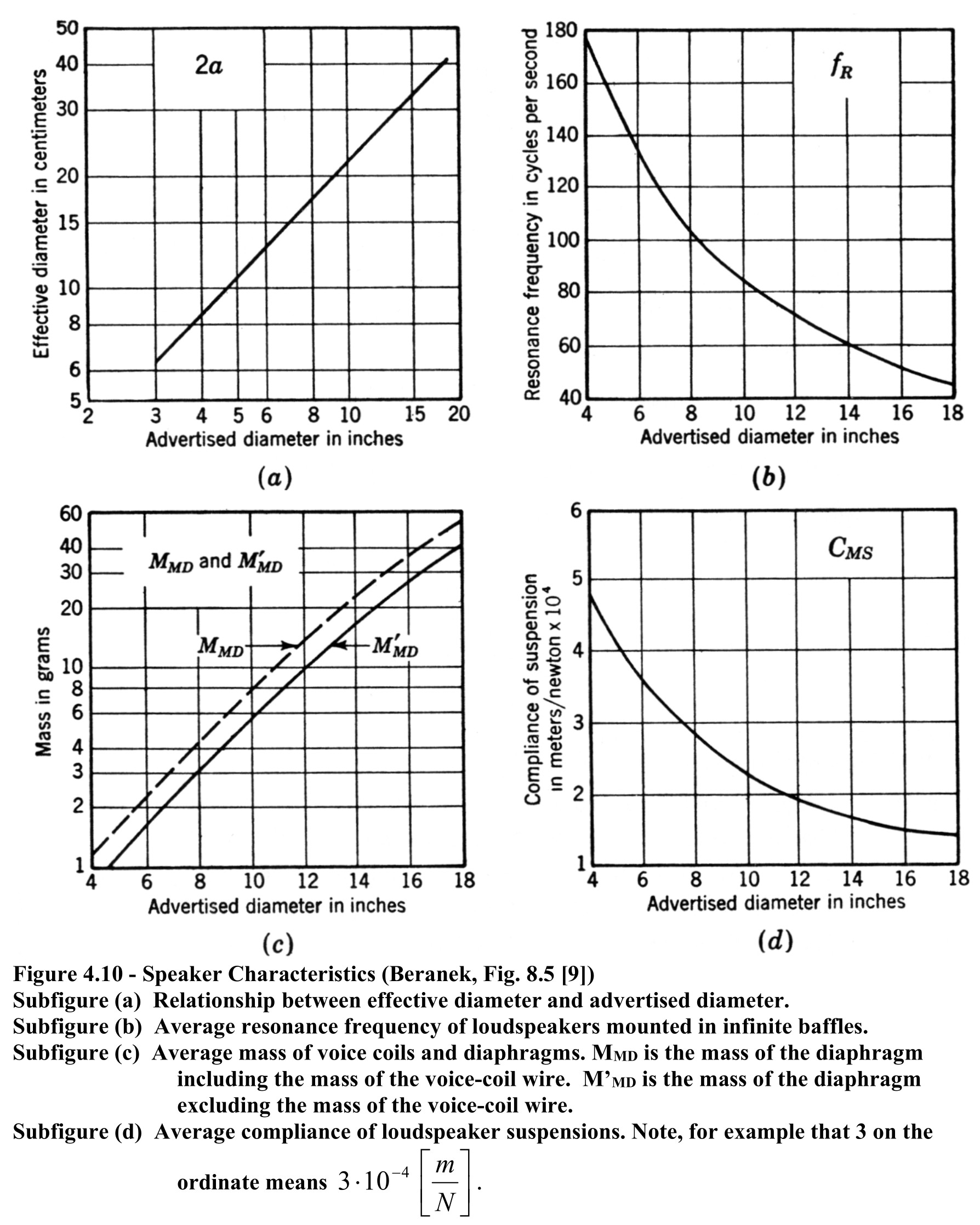
The acoustic frequency range covers 3 decades, running from 20 Hz to 20,000 Hz. However, the frequency response for a moving coil loudspeaker is flat over a 1-decade range. Thus, most high-quality speaker systems consist of at least 3 moving coil loudspeakers. Most audiophiles now seem to insist on at least 4 drivers. Table 4.3 gives the range of flat frequency response for typical loudspeakers found in a speaker system.
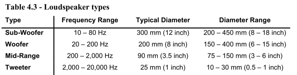
Leo Beranek [9] provides values for loudspeaker parameters determined experimentally. His Figure 8.5 is shown in Figure 4.10.
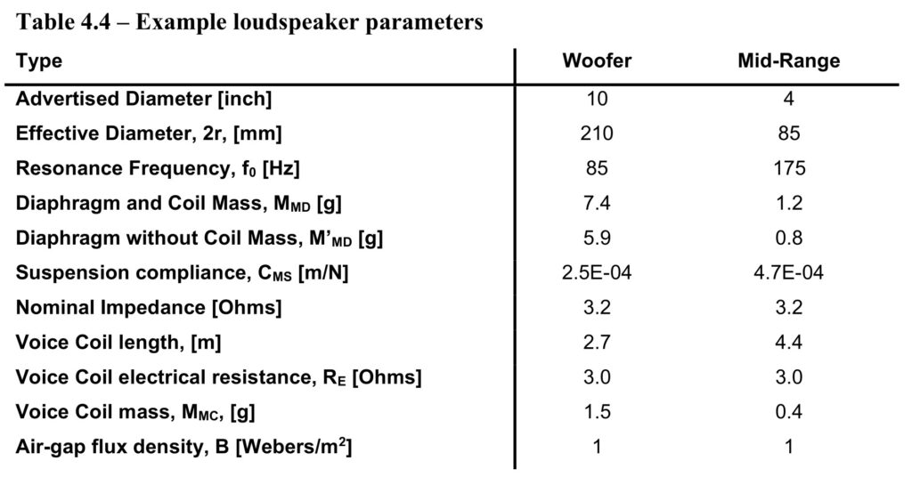
From Figure 4.10, and [9] values for a typical woofer and midrange are shown Table 4.4.
Loudspeaker without Enclosure
The previous section concerned loudspeakers in an infinite baffle. A speaker mounted in a large stiff wall is generally a good approximation to an infinitely baffled speaker. The speaker frequency response is affected by its enclosure. But, before looking at the effect of various enclosures, consider the case without an enclosure – a loudspeaker in free space, as illustrated in Figure 4.11.
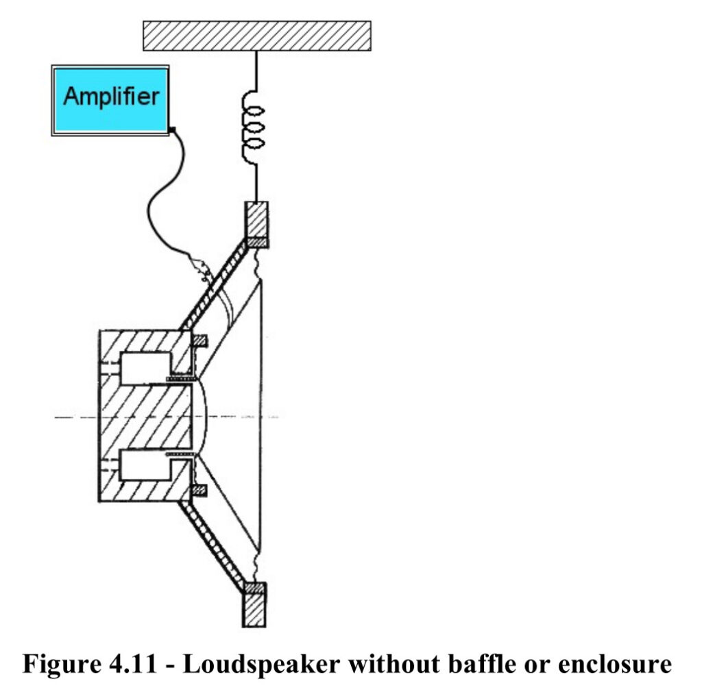
With no baffle, the radiation from the front and rear faces of the loudspeaker is an acoustic dipole whose on-axis output is

with

Below the fundamental resonance frequency

Thus below the resonance frequency

so the slope of the TVR is 18 dB/octave at low frequency.
Above the fundamental resonance frequency

giving

and therefore the slope of the TVR equals 6 dB/octave at high frequency.
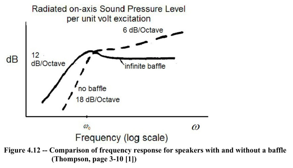
Figure 4.12 compares the TVR shape of a loudspeaker without a baffle to the shape shown in Figure 4.9 for a loudspeaker in an infinite baffle. To allow easy comparison, the dB references were adjusted so the curves match at the resonance frequency. The advantage of having a baffle is evident in Figure 4.12. Notice that the response above the resonance frequency for the unbaffled case is not flat.
Closed Box Baffle
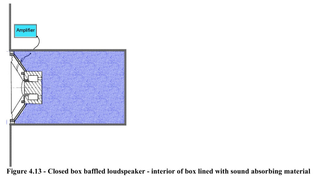
Figure 4.13 schematically shows a loudspeaker at one end of a closed box. To discourage standing waves in the box, it is lined with a sound absorbing material.
The enclosure is reminiscent of the closed tube shown in Figure 2.2, which is repeated in Figure 4.14.
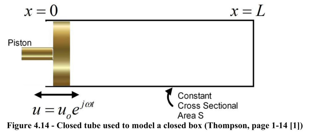
Thus, the acoustic impedance of the closed box, ZAB, is given by

The sound absorbing material adds acoustic resistance, RAB.
The system in Figure 4.13 is modeled by starting with a bond graph used to model the speaker. Since only the acoustic part of the device is different, start with the version of the bond graph shown in Figure 4.7d, then add the acoustic damping of the enclosure filler material (element R722), and the box impedance (element D723) as shown in Figure 4.15.
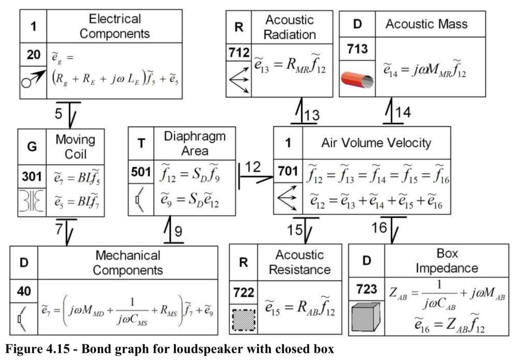
Elements 712 and 713 represent only one side of the speaker so do not have the factor of 2 used with elements 602 and 603 in Figure 4.6. Elements 722 and 723 provide the forces imposed on the other side of the loudspeaker.
Figure 4.15 gives all the information needed to determine the TVR for the loudspeaker with a closed box, but like what was done to develop the simplified bond graph in Figure 4.8, the bond graph in Figure 4.15 can be reduced, to determine the fundamental resonance frequency of the device.
Recall that for the frequencies of interest, LE is set to zero and then group the terms in the elements in Figure 4.15 by separating the real and imaginary values. These actions give Figure 4.16.
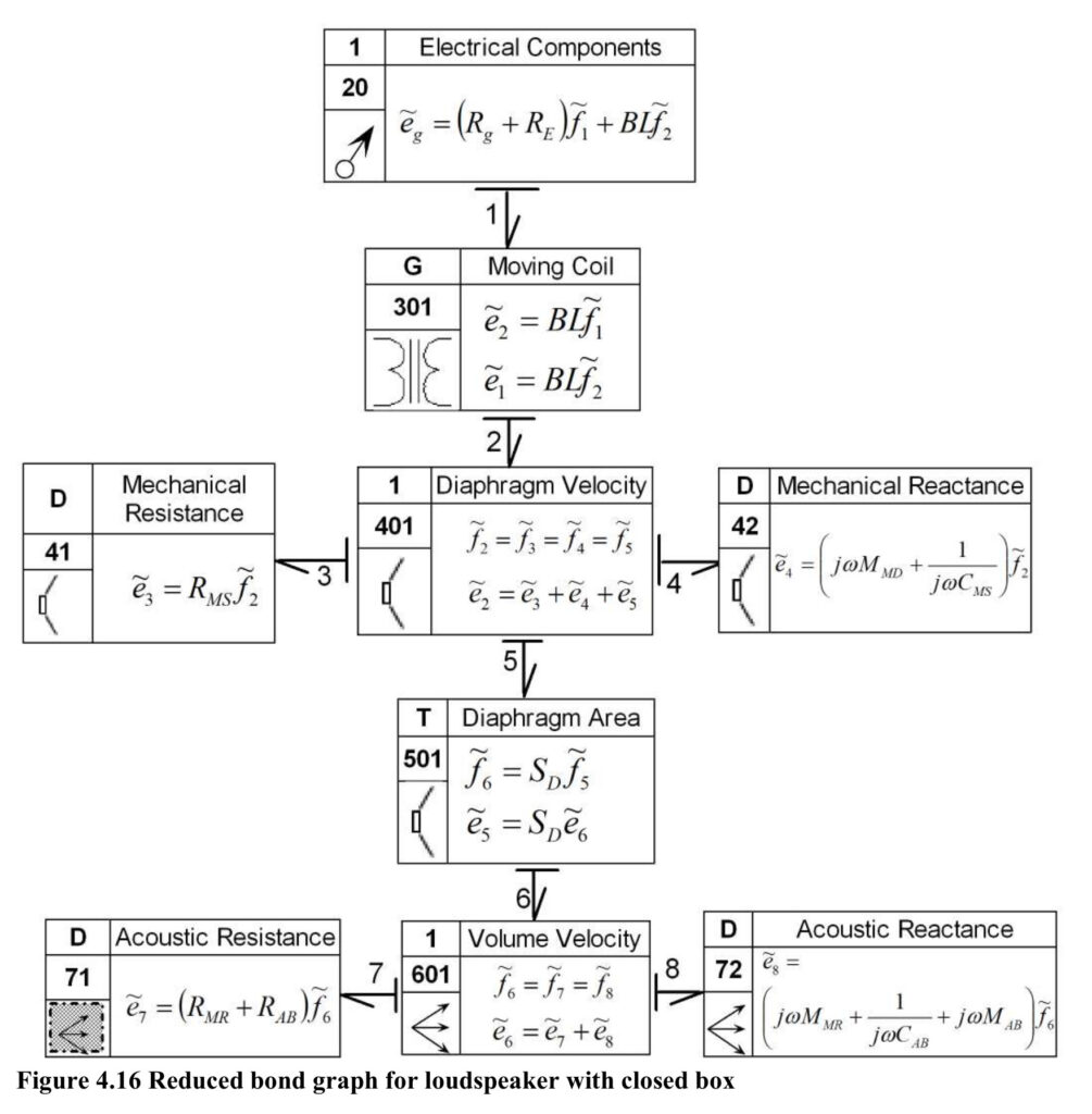
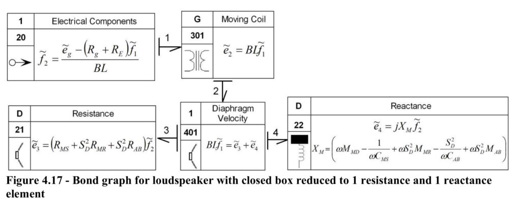
The bond graph is simplified by using the gyrator and transformer relationships to eliminate variables to give Figure 4.17.
The undamped Resonance frequency,
can be
determined from the equation for XM in element D22 in Figure 4.17. A resonance occurs when

From the figure and {4.68}

thus

Solving {4.70} for
gives
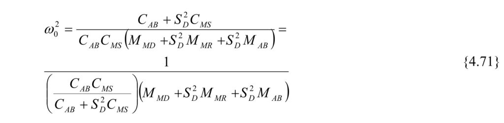
For a speaker with a closed box. It would be nice to know if adding the box increases or decreases the resonance frequency compared to a baffled speaker without a box.
Equation {4.54} provides

Dividing {4.71} by {4.72} gives
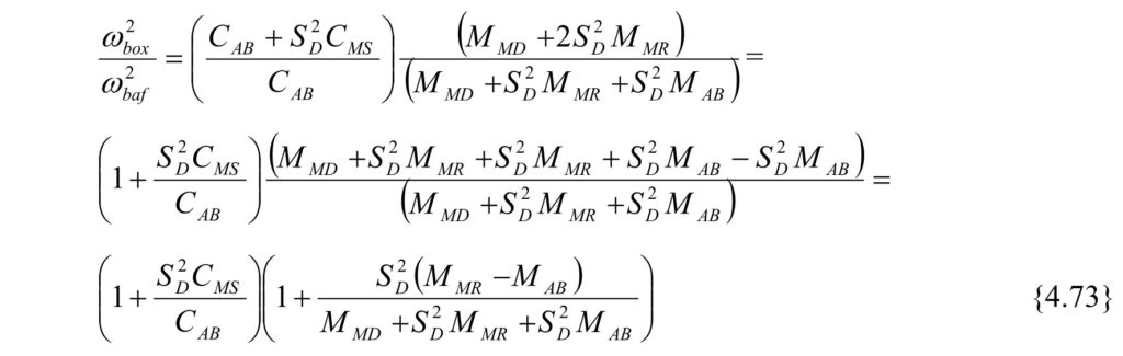
Equation {4.73} shows that the frequency ratio,
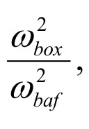
is greater than 1 if

Beranek [9] provides a relationship for determining the acoustic mass for a loudspeaker in a closed box with an absorptive lining

where a is the effective piston radius of the loudspeaker, and BML depends on the ratio of the piston area, SD, to the area L2 of the side of the box in which it is mounted. His Figure 8.6, is shown in Figure 4.18.
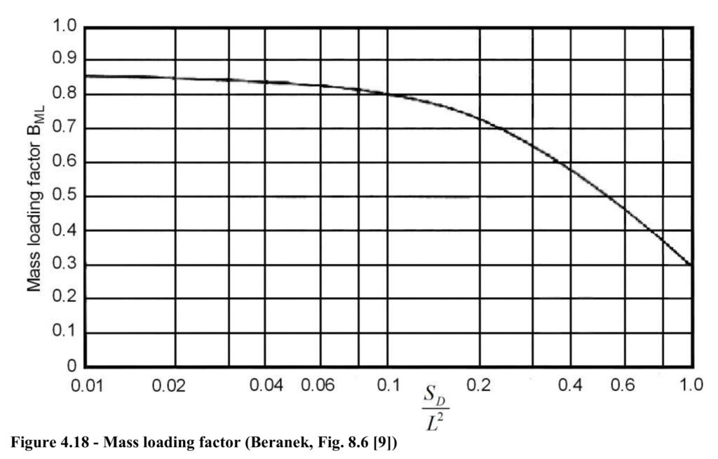
The graph shows that the value of BML approaches 0.849 when the piston area is small compared to the face dimension of the box. MMR is equivalent to a small loudspeaker in a very large box, thus

Likewise from Figure 4.18, the acoustic mass MAR for the speaker in the box is

therefore

which gives

Radiated Sound Pressure from a Loudspeaker in a Closed Box
Since the radiated power is related to the acoustic resistance, RAB, by


Then

where for low ka:


Since the acoustic radiation behavior of a loudspeaker in a closed box is somewhere between the behavior of a loudspeaker in a tube and a baffled loudspeaker

The directivity factor for a loudspeaker in a tube and a baffled loudspeaker varies with wavelength as shown in Figure 4.19.
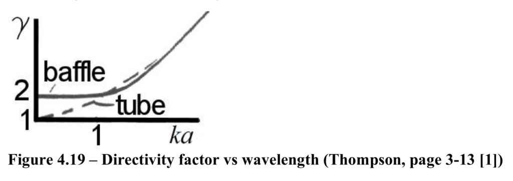
For ka < 1.5

For ka > 1

therefore

Below the principal resonance frequency where the behavior is stiffness controlled


Therefore

and

Above the principal resonance frequency where the behavior is mass controlled

and

So invoking {4.78}

Since {4.95} indicates one factor in {4.82} is greater than 1, and {4.88} indicates that another factor is less than 1, the pressure ratio relationship is not clear above the principal resonance. As shown in Figure 4.20, it turns out that in this situation

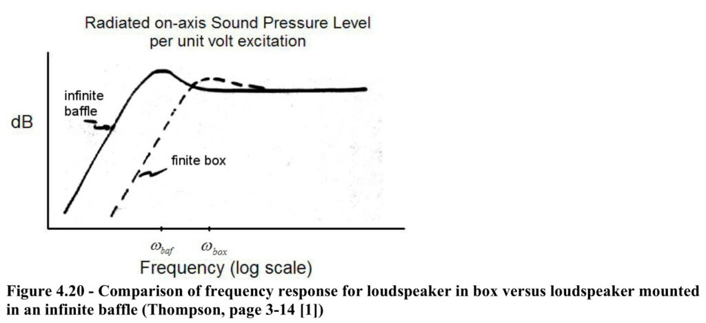
As the speaker box gets bigger, the frequency response curve moves to the left getting closer to the infinite baffle case. The height of the finite box curve at the resonance frequency depends on the damping value, QM, given by {4.57}.
Acoustic Suspension Speaker
Closed box speakers with a soft mechanical suspension, i.e. large CMS, are called acoustic suspension speakers. The diaphragm and voice coil are often more massive than those used with ordinary speakers, hence the unbaffled resonance frequency is in the 10-20 Hz range. Sealing the components in a closed box, raises the fundamental resonance frequency to approximately 40 Hz. The efficiency of these speakers is lower than conventional speakers, so a larger magnet is used to increase the magnetic strength, B.
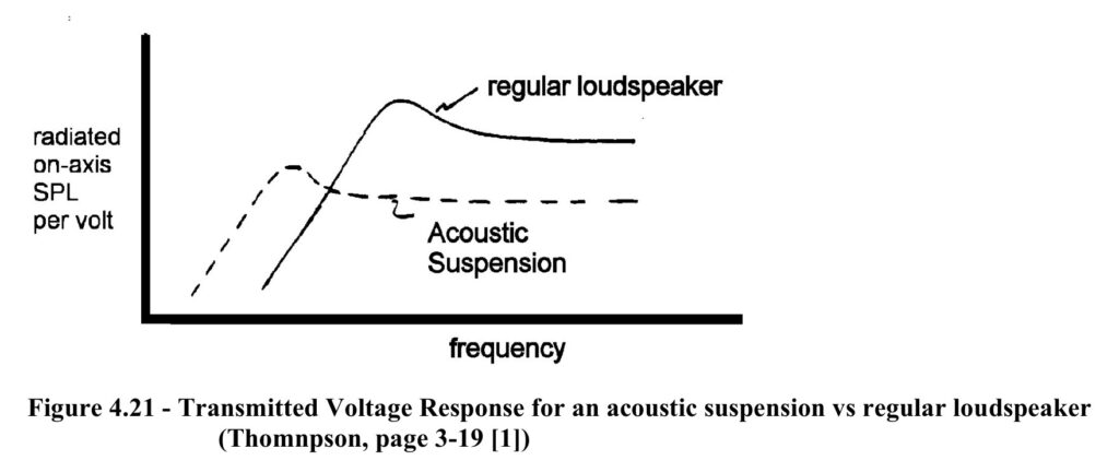
Frequency response analysis of acoustic suspension speakers is the same as for closed box speakers, however for the same diameter loudspeaker, and same size enclosure, the resonance frequency is lower as shown in Figure 4.21. Note the magnitude of the frequency response is also lower, hence lower sound radiation efficiency.
Bass Reflex Enclosure
Figure 4.22 shows a commonly used enclosure called a bass reflex speaker.
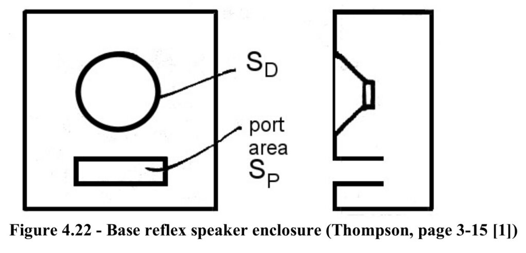
Alternative names include vented or ported enclosure.
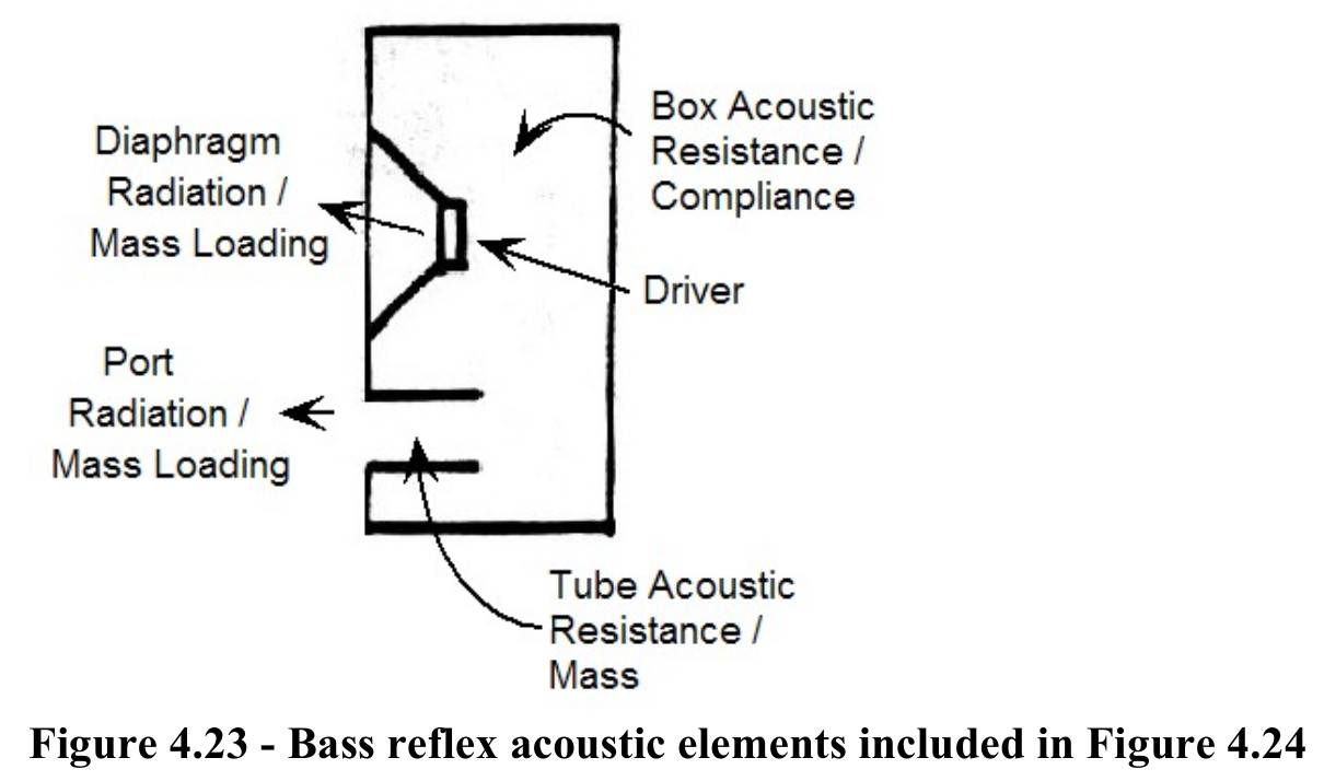
The tube that leads to the port has an acoustic mass, MAP, and an acoustic resistance, RAP. The port outlet has radiation resistance, RARP, and acoustic mass loading, MARP. The box provides acoustic compliance CAB, and the lining in the box provides resistance, RAB. At the low frequencies considered in this analysis, the acoustic mass, MAB, of the air in the box can be ignored. Figure 4.23 shows the acoustic elements that are included in the bond graph tile for the acoustic part of the speaker shown in Figure 4.24.
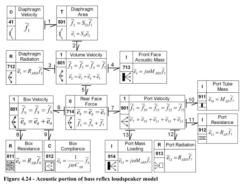
Figure 4.24 shows there are two sources of acoustic radiation. For low frequency as given by {4.83} and {4.84} the radiation resistance is independent of geometry, thus RARD in element R712 has the same value as RARP in R913. Rename this parameter RAR.
Again use the power relationship

to obtain the radiated pressure. The radiated power is not the sum of the power flowing to the two acoustic radiation elements. The volume velocity on the front face of the diaphragm is exactly out of phase with the volume velocity from the rear face of the diaphragm that drives the port radiation. The net effect on the far field pressure is a partial cancellation. The net radiated power is therefore

Element 0714 shows that

Thus the radiated acoustic pressure is

The directivity factor, γ, is dropped from {4.100} since low frequency radiation is omnidirectional, i.e. γ=1.
Recall from {4.83} and {4.84}

Thus from {4.100}

Since damping does not change the number of resonances, or the slope of linear sections of the frequency response, if just the frequency characteristics of UB, are of interest, the bond graph in Figure 4.24 can be simplified by neglecting all the resistance elements, combining like elements, and eliminating transformers and gyrators. The bond graph shown in Figure 4.25 provides the simplified model, with all parameters in the acoustic domain.
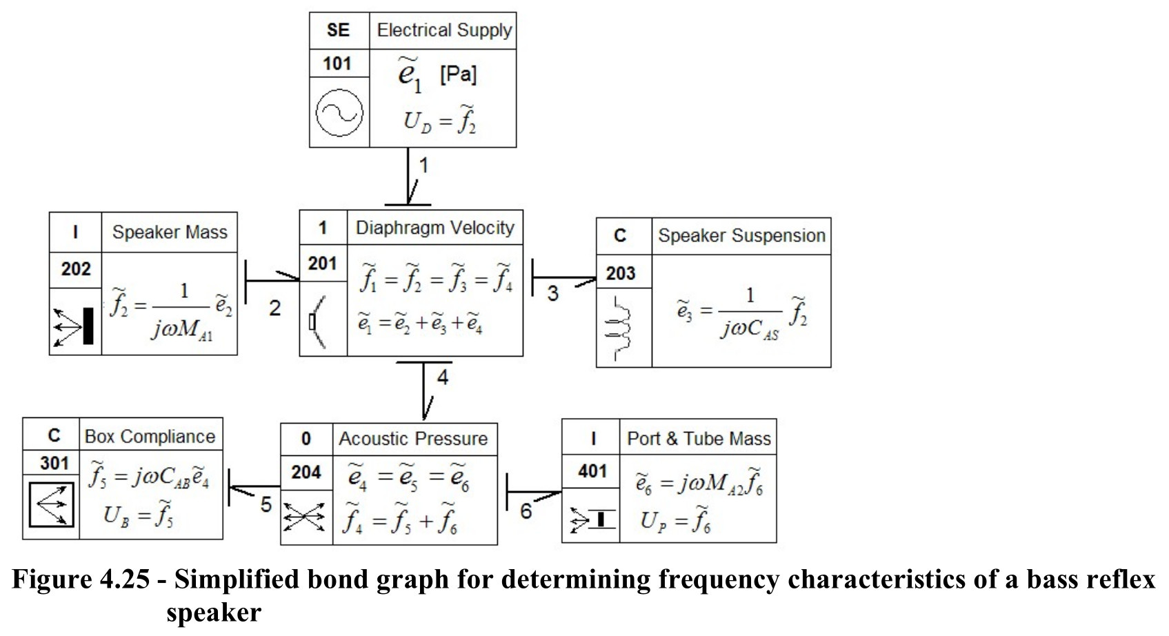
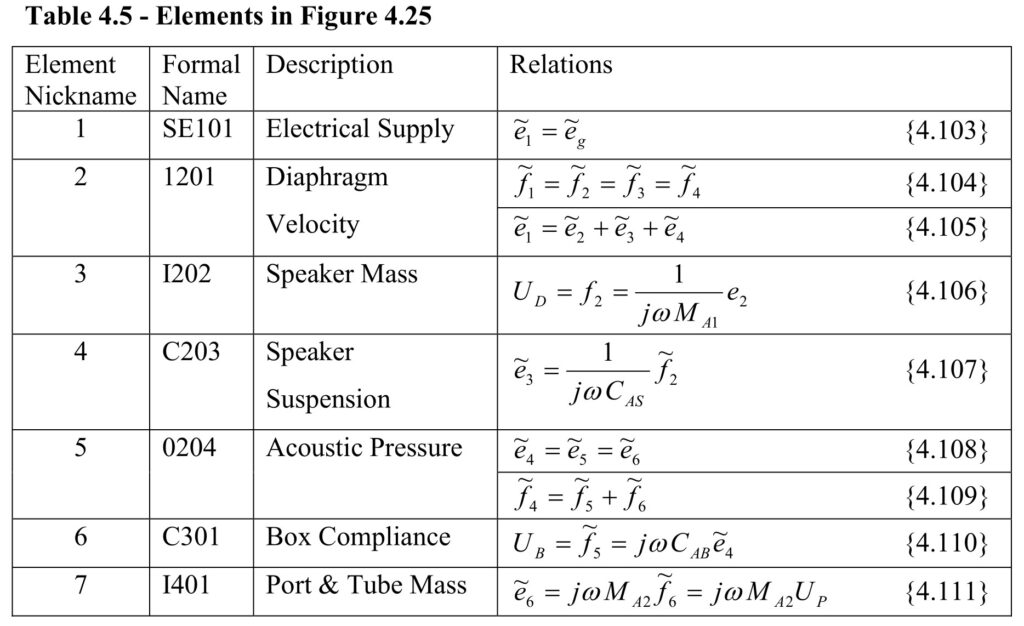
From {4.105}

Substituting element equations from Table 4.5 gives


From {4.109}

From {4.108}

Solving
then

giving

Then from {4.114}

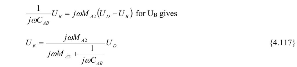
Equation {4.117} can now be solved for UB to give

Since
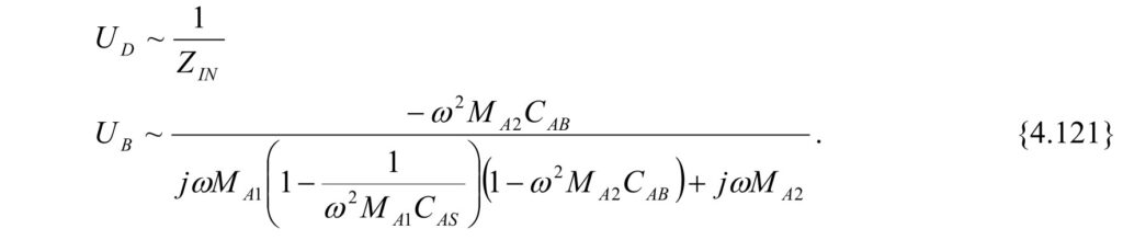
Then
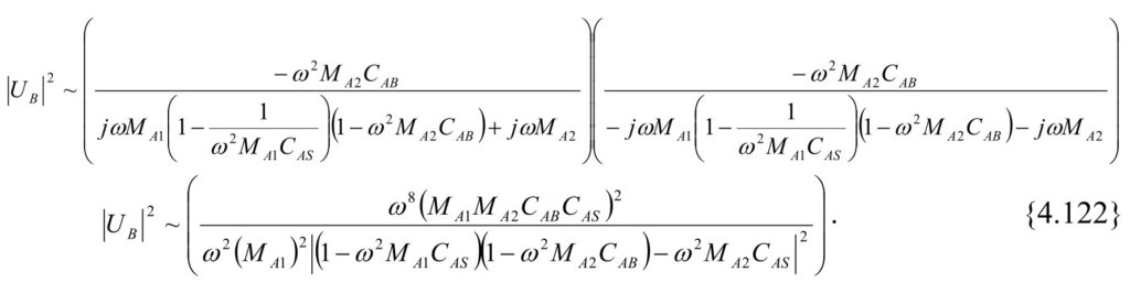
Hence

Since

at low frequency the sound pressure from a bass reflex speaker has frequency response

As with earlier examples, a resonance frequency, ω1, can be determined by considering when the denominator for Z4 is zero, that is


For this condition
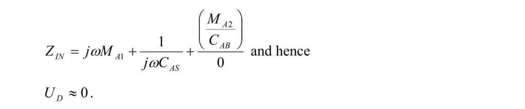
So, from {4.115} at first glance it would appear that UB and thus UP
would be small. However,
is not zero (it is undefined).
UP can be large, giving a large amount of radiation from the port, even though the radiation from the diaphragm is small.
Speaker designers tend to choose

that is approximately the resonance frequency of the speaker in an infinite baffle.
Above ω1, the impedance
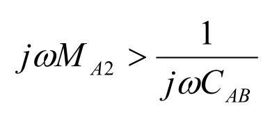
and the box starts
to behave as if there were no port.
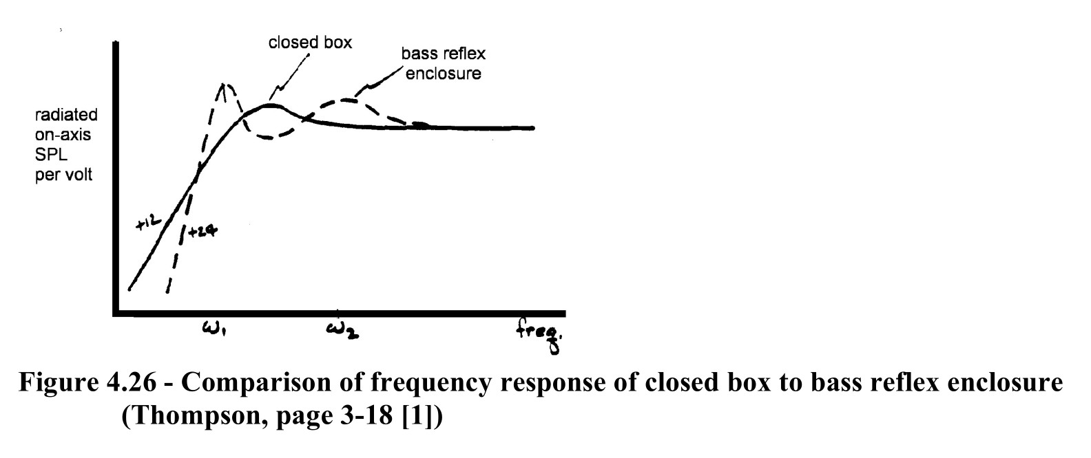
There is another resonance, ω2, when ZIN is zero. The effective compliance is slightly less than the series combination of CAS and CAB, thus ω2, is greater than the principal resonance frequency of the speaker in the same sized closed box. Above this second resonance, the port is effectively blocked, and the response is the same as for a closed box speaker. Figure 4.26 compares the frequency response of a bass reflex speaker with a closed box speaker.
Horn Loudspeakers
Another approach to get more output at low frequencies is to attach a horn to a small diameter moving coil driver. The horn is an acoustic transformer that matches the impedance of the air to the impedance of the driver, increasing the resistive radiation loading on the driver, and hence increasing the low frequency acoustic output. Horn speakers have more directivity than enclosed speakers and are often used in outdoor venues such as stadiums. The length of the horn and the resultant large size is a disadvantage. Figure 4.27 shows a schematic of typical driver and horn.
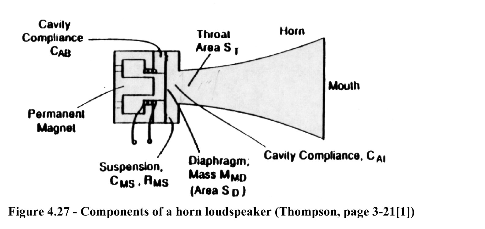
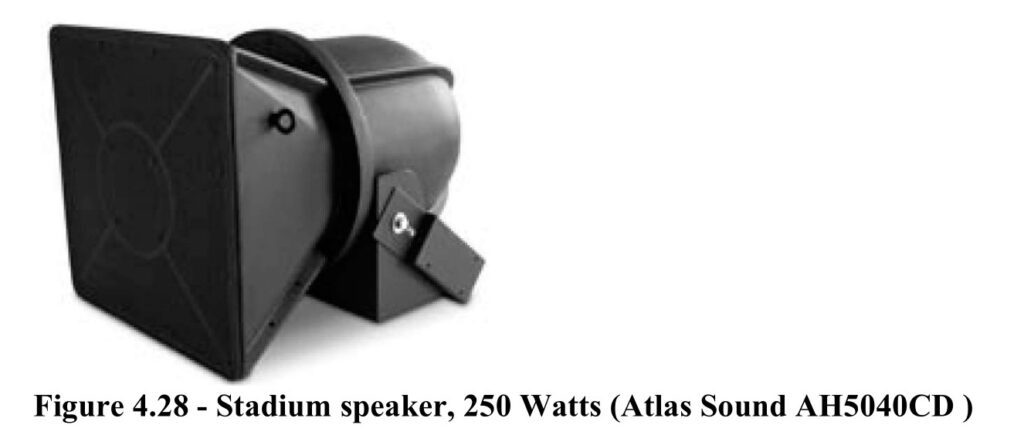
Figure 4.28 shows a stadium loudspeaker with a frame woofer and a concentric 50˚H x 40˚V horn.
The small end of the horn is called the throat. The large end is called the mouth. The rate of change of area with length is called flare.
The following assumptions are made for analyzing horn behavior:
- Linearized acoustic equations are applicable (true for typical sound pressure levels)
- Plane waves propagate parallel to the horn axis; i.e. there is no particle motion perpendicular to the axis. Pressure and velocity are only functions of time and axial distance, x. (true at low frequency)
- Horn walls are perfectly rigid
- Horn flare is sufficiently gradual that the assumed plane waves do not lose contact with the walls
The linearized small signal acoustic wave equation for the harmonic time dependence pressure at any point along a horn is:

Equation {4.128} can be expanded to give the following two equivalent relationships


Horns of several shapes can be analyzed. As an example of the approach, the response of speakers with exponential shaped horns will be developed in the following section.
Exponential Horn
The cross-sectional area of an exponential horn is given by

where S0 is the area at x=0, and m is the flare constant.
Taking the logarithm of both sides of {4.131} gives

Therefore,

Substituting {4.133} into {4.130} gives

With the trial solution

So {4.134} is equivalent to

For {4.135} to be a trial solution, equation {4.136} requires

Solving for G, gives

with

A more general solution is a linear combination of the two solutions, thus {4.135} becomes

The first term is a right propagating wave, and the second term is a left propagating wave. This function describes a plane wave with exponentially decreasing amplitude. The attenuation is due to the wave spreading over an increasing cross-section as it propagates.
From {4.139}, β, the effective wave number, is given by

The corresponding effective phase velocity,
is

When
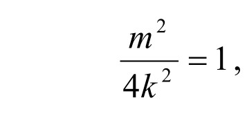
the effective phase velocity
and β = 0
This condition occurs at the cutoff frequency, fc.

For f < fc , β is imaginary and therefore –jβ is negative real. Hence there is no radiation, just an exponentially damped wave. In other words, for a propagating wave, the flare coefficient, m, must satisfy

The particle velocity amplitude,
is related to the pressure
amplitude by

and the volume velocity amplitude, Ũ, is related to the particle velocity amplitude by:

The acoustic impedance at any point x in the horn can be determined from
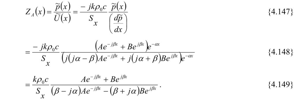
The coefficient A depends on the amplitude of outgoing waves. Coefficient B accounts for the incoming waves. If the horn is in a free field, the only incoming waves would result from reflections off the end of the horn. For an infinitely long horn, there would be no reflections, and B = 0. Kinsler and Frey [7] state that the amplitude of the reflected wave is small compared to that of the incident wave (B<A/10) whenever the radius of the mouth, aL, satisfies

and for such horns, the length can be considered infinite.
For an infinitely long horn, B=0. Therefore,

At the throat, x=0, and

Equation {4.152} shows that ZA has both an acoustic resistance term (real), and an acoustic reactance term (imaginary). For frequencies above the cutoff (the only frequencies of interest here), the acoustic resistance increases with frequency, and the acoustic reactance decreases with frequency.
A reactance component with characteristics like

may be unfamiliar. Thompson[1] calls it a negative capacitor.
The acoustic impedance at the throat of the horn can thus be written as

with

and

Kinsler and Frey [7] compares the acoustic resistance and the acoustic reactance at the throat of an infinite exponential horn with values for a piston of the same size mounted in an infinite baffle. Their Fig. 14.19 is shown in Figure 4.29.
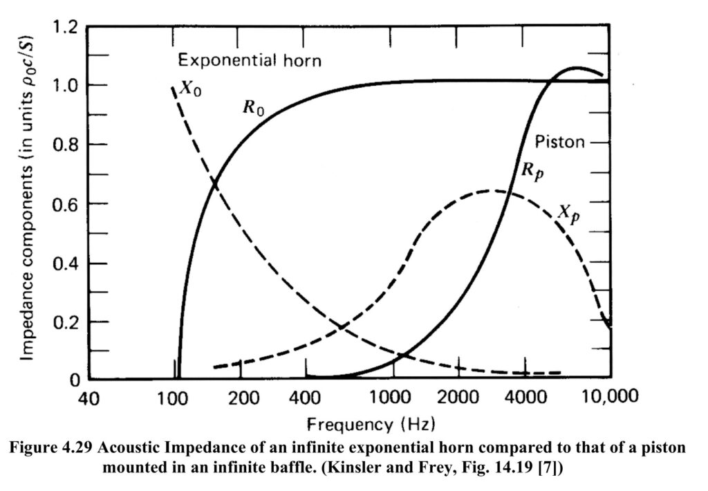
For the conditions shown in Figure 4.29, in the frequency range from 100 to 3,000 Hz the radiation from the horn is greatly enhanced since the resistance loading at the throat of the horn is significantly greater than that on the piston mounted in an infinite baffle.
Frequency Response of Speaker with an Exponential Horn
Figure 4.30 conceptually shows a horn speaker with the components that will be included in its system model.
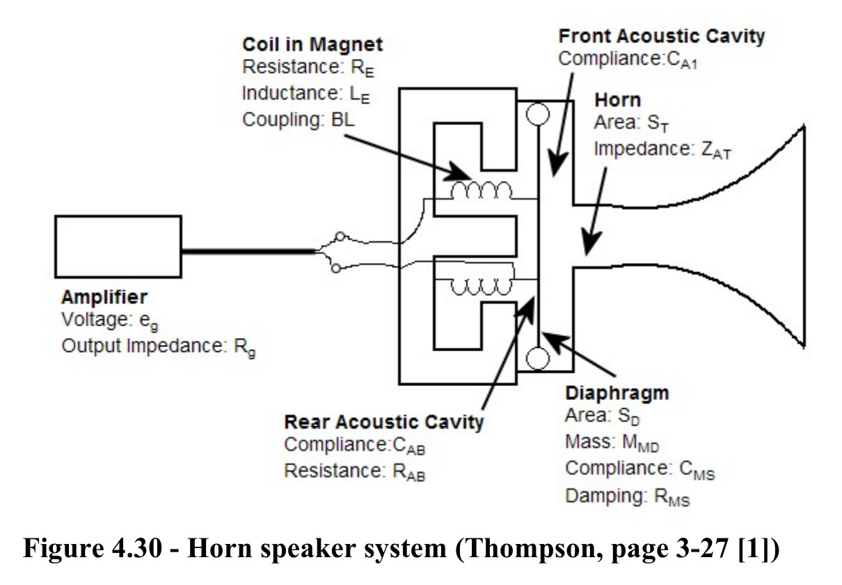
From the amplifier to the diaphragm, the model is identical to that developed at the start of this chapter for a moving coil loudspeaker.
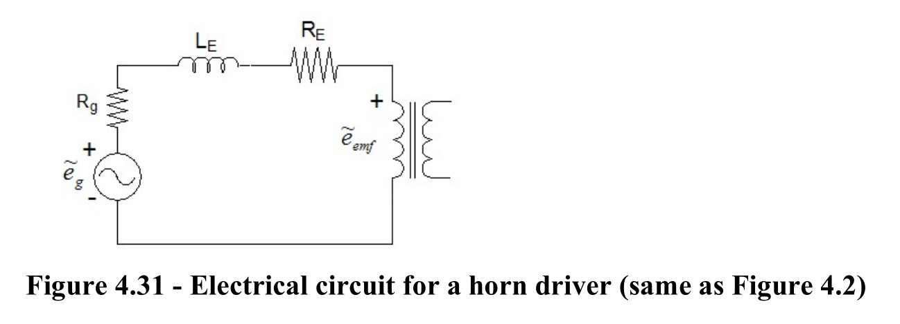
The amplifier is considered an effort (voltage) source in series with a resistance, Rg. The current from the amplifier flows through the coil suspended in a magnet. The coil has inductance LE, and resistance RE. The coil with an oscillating current in a magnetic field generates a force on the diaphragm, and the moving coil generates a back emf in the electrical circuit. Figure 4.29 shows the electrical circuit, and Figure 4.30 shows a bond graph tile for the circuit.
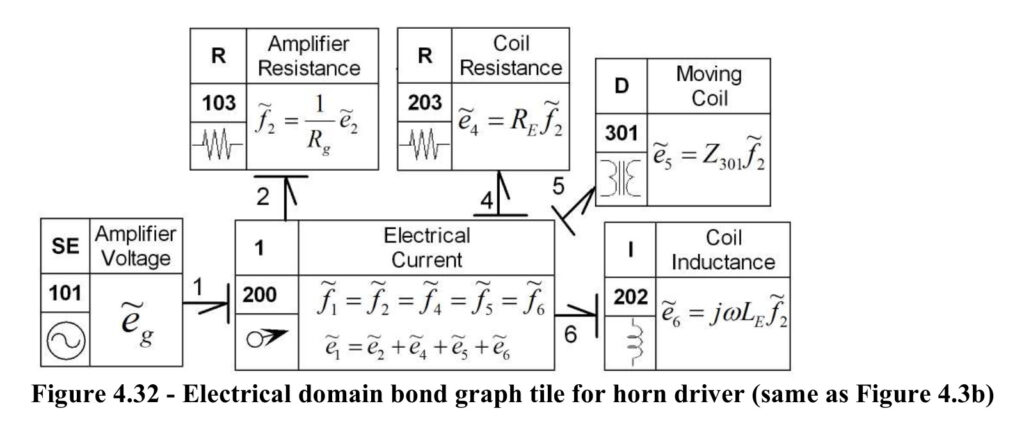
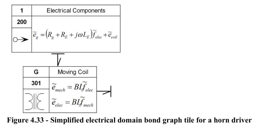
Using a method similar to that used to generate Figure 4.7, the bond graph in Figure 4.32 is reduced to 2 elements giving Figure 4.33.
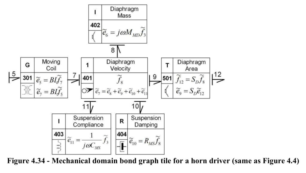
The moving coil gyrator converts the electrical current to a force on the diaphragm to drive the mechanical components shown in the bond graph tile given in Figure 4.34.
The acoustic domain has 3 components.
- The sealed volume behind the diaphragm provides acoustic compliance and acoustic resistance
- The volume between the front face of the diaphragm and the horn throat provides acoustic compliance
- The horn throat provides an acoustic impedance with an acoustic mass component and an acoustic resistance (radiation) component as given by {4.142}
Figure 4.35 shows the acoustic domain bond graph tile.
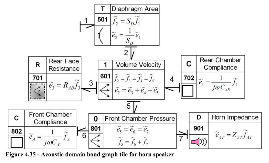
Figure 4.35 – Acoustic domain bond graph tile for horn speaker
Since the rear chamber is sealed, its behavior affects the diaphragm suspension characteristics. The effects can be considered part of the suspension by converting its acoustic domain characteristics to the mechanical domain.
Figure 4.36 shows the combined mechanical and acoustic domain bond graph tiles ready for transforming the rear chamber characteristics to the mechanical domain.
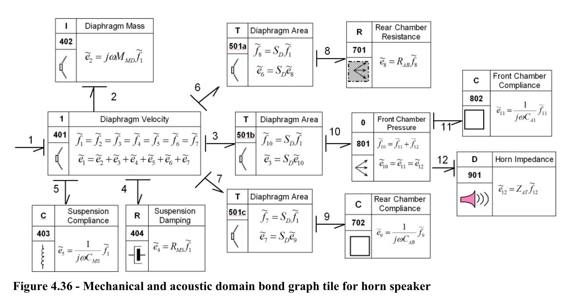
By taking T501a, and T501c into R701 and C702, Figure 4.36 is reduced to give Figure 4.37.
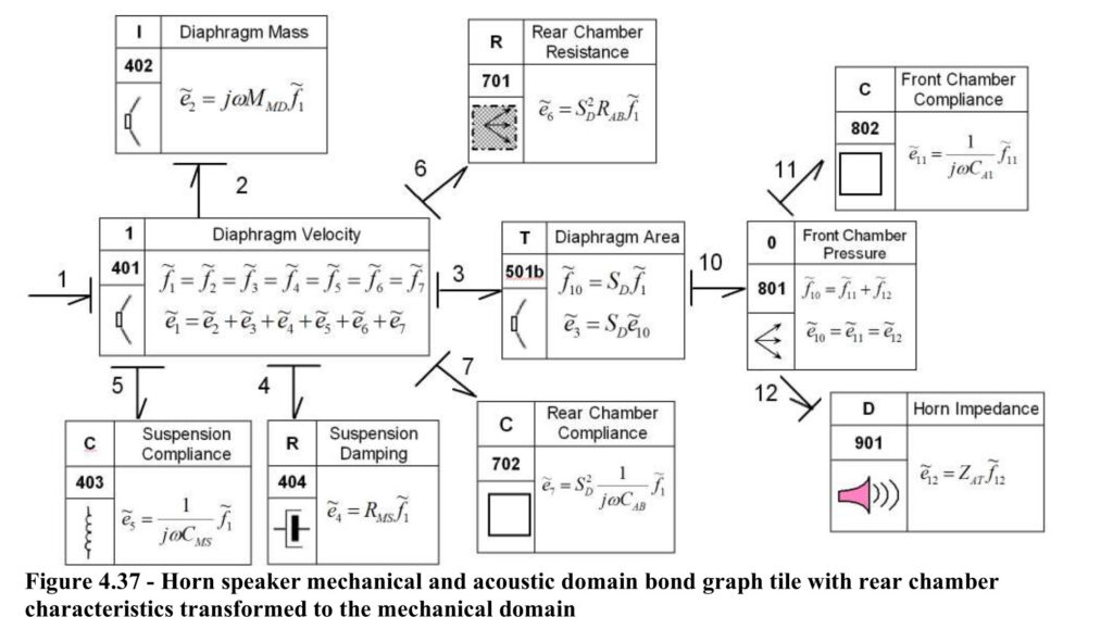
Figure 4.37 can be simplified by bringing the mechanical 1-port elements into 1401, and the acoustic 1-port elements into 0801 as shown in Figure 4.38. As mentioned for the moving coil loudspeaker, at the frequencies of interest, the coil inductance can be ignored.
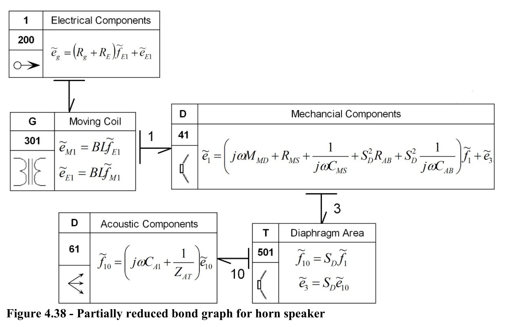
The gyrator and the transformer can be eliminated by using mechanical equivalents for each of the efforts and flows. T501 gives the relationship between the diaphragm velocity
amplitude,
and the volume velocity amplitude,
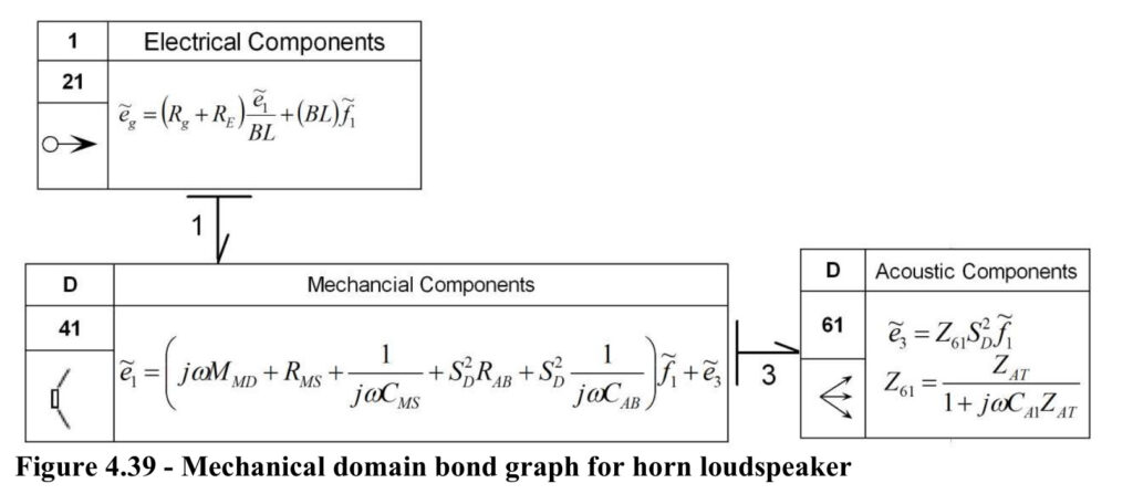
From element 121 in Figure 4.39

From element D41 in Figure 4.39

From element D61 in Figure 4.39

Substituting {4.158} and {4.159} into {4.157} gives

or

From Figure 4.39

then

Since from {4.154}
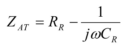
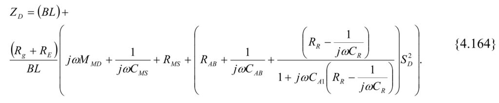
Let
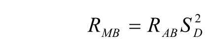
and
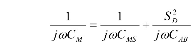
Then {4.164} simplifies to

The sound power radiated from the horn, WH, is given by

and

where
where ũT is the particle velocity amplitude in the throat of the horn.
From 0801 in Figure 4.37
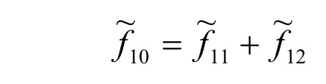
or

Since Ũ = Sũ
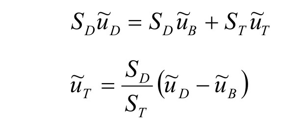
The above equations provide the relationships needed to determine the characteristics of the frequency response magnitude.
Low Frequency Behavior
At very low frequencies, the compliance of the front chamber can be ignored. Thus
and
From {4.161} and {4.165}


At low frequency, since the mechanical mass of the diaphragm, MMD, is small, to have a reasonably low resonance frequency the compliance of the mechanical suspension, CMD, must be large, therefore MMD can be neglected. Also at low frequency, jωCA1 can also be ignored, thus
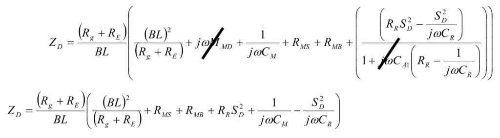
and

Since RR, the radiation resistance of the horn, is a function of
frequency, the term with
can be substituted with
For purposes of understanding the low frequency characteristics of {4.171} the constants can be adjusted so
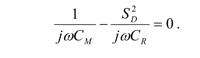
So {4.171} becomes

where

Recall the radiated power is given by

Then with {4.173} and {4.174}, the form of the horn power can be identified in this frequency range

From {4.155}

and thus for low frequency RMR is imaginary, so no radiation would be expected. However, when doing these types of approximations, it is best to just assume RMR is a constant.
When the mouth of the horn is large compared to the wavelength, the directivity function of a horn is proportional to the square of the frequency.
Thus from {4.167}

The low frequency range ends near the principal resonance frequency, ω0, so the next task is to solve for it considering the reactance terms in Figure 4.39.
Principal Resonance Frequency of Horn Loudspeaker
Similar to the procedure followed with Figure 4.15 to get Figure 4.16, the behavior of the reactance terms can be estimated by ignoring the resistive terms and the transformations in {4.165}. Figure 4.40 is a conceptual bond graph showing the relationship of the components that affect the principal resonance frequency. The horn impedance has been simplified to only include the negative compliance.
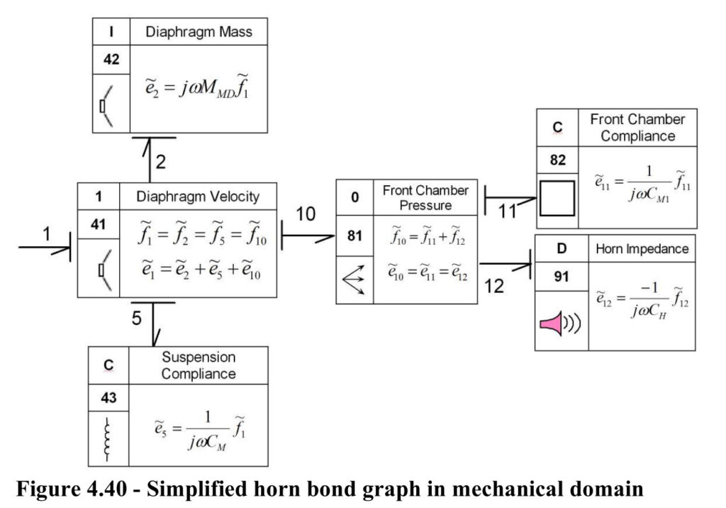
Element 081 provides an effective compliance for the sum of C82 and D91.

Using the Element 141 relationships, the total effective compliance is given by

where

The parameters can be selected so CM ≈ CH giving

and

Above the Principal Resonance Frequency
The complete bond graph for the horn loudspeaker is shown in Figure 4.41.
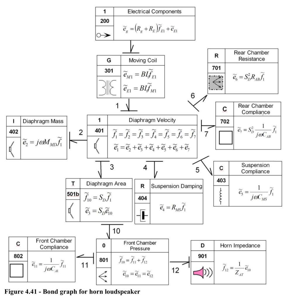
From Elements 1200 and G301, the expression for the mechanical force on the diaphragm, ẽ1, is

From elements I402, C403, R404, R701, C702 and 1401

Recall

then {4.184} can be rewritten

Thompson [1] sets

by arguing that since MMD is small it can be ignored. He further ignores the effect of CM by considering just the case with CM = CR.
Then

Removing T501b by taking the transformer relationships into the elements C802 and D901 allows Figure 4.41 to be simplified to give Figure 4.42.
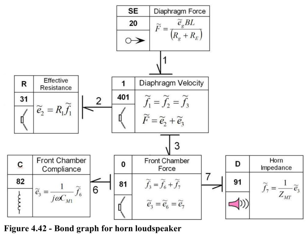
The equations in Figure 4.40 give the horn flow,
as:
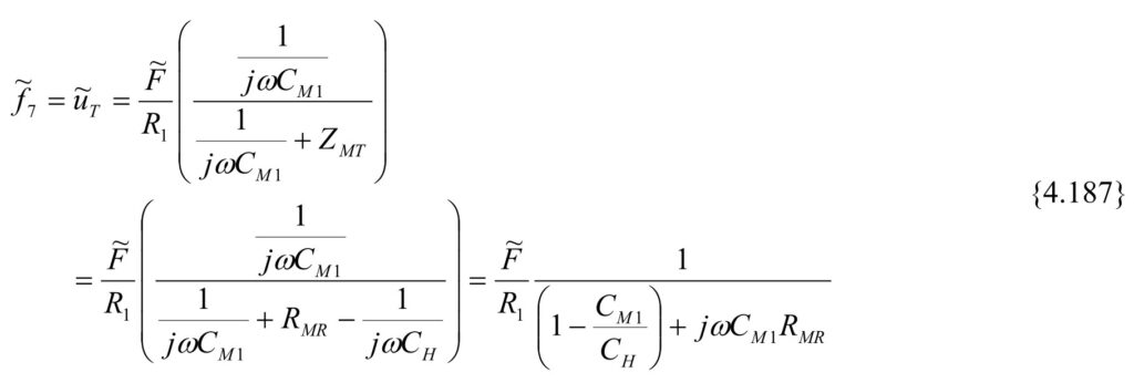
then by setting the effective compliance of the horn to the effective compliance of the driver, {4.187} reduces to

The acoustic radiated power is

Recall that for a large (compared to the wavelength) horn the directivity is proportional to the square of the frequency,

and thus the on-axis sound pressure level is given by

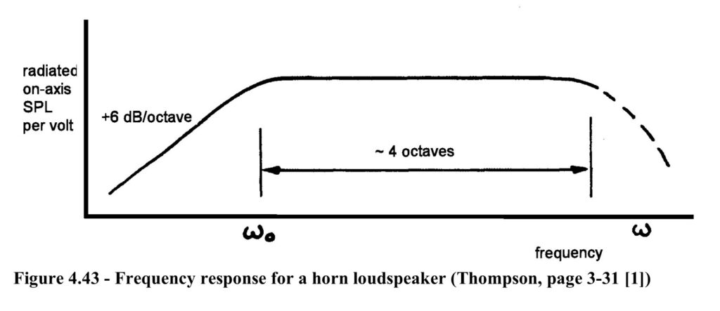
The heavy resistance loading caused by the horn gives a flat frequency response that extends about 4 octaves as shown in Figure 4.43
Single-sided Electrostatic Speaker
Another concept for speakers involves using a thin membrane as a diaphragm. The diaphragm is moved using electrostatic forces. The force of attraction between two charged plates, Eelectrostatic, shown
as
in Figure 44 is given by Coulumb’s Law
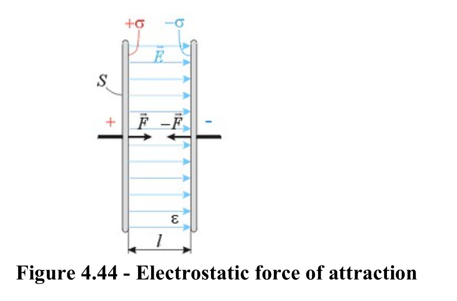

where
ε0 is the dielectric constant for air
S is the surface area of one plate
E is the voltage between the plates and
ℓ is the distance between plates.
Since the voltage is squared, the force is always positive (attraction), even if the voltage is negative. If the force is constant, then varying the voltage causes the separation distance, ℓ, to vary.
Let ℓ=d+x and E=E0+Asin(ωt). Figure 4.45 shows the non-linear relationship between the voltage, E, and the displacement, x, when Eo is zero. The fundamental frequency of the output is twice that of the input.
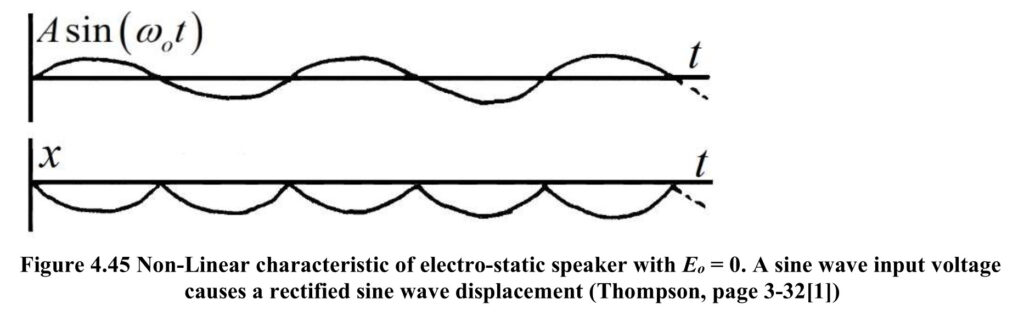
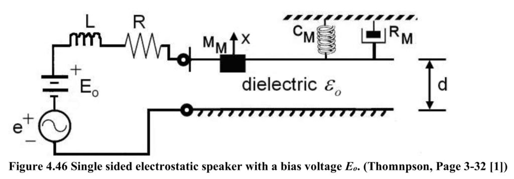
Figure 4.46 shows a conceptual model of a single sided electrostatic speaker. The electrical circuit has a static and dynamic voltage source, an inductor and a resistor. The mechanical components include one moving plate with mass and a compliant suspension with damping.
From {4.192} the attraction force is proportional to the square of the voltage

For E0>>e the last term can be ignored and the force is linear in e.

With the membrane moving in air, there is also a force, ediaphragm, on the membrane due to the acoustic radiation. The differential equations for the diaphragm and the electrical circuits are


Although bond graphs and numerical simulation can handle the coupled non-linear equations given in {4.194} and {4.195} a good model can be obtained by linearizing the equations by assuming that the state variables consist of a DC term plus an AC term.
Let
and with e and ediaphragm in {4.194} and {4.195} being only AC.
Also denote
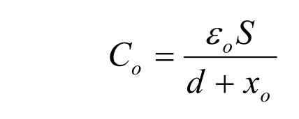
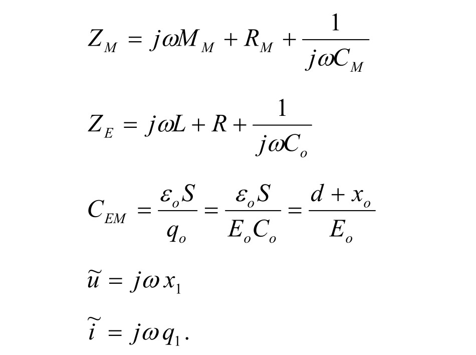
Then equating the DC terms, and the AC terms and keeping just the 1st power of ω terms equations {4.194} and {4.195} give 4 relations:
- The charge-voltage relationship for a capacitor

- An expression for the equilibrium value for xo

- And the AC terms


Normally the equations would be developed from the bond graph, but in this case, the relationships in the equations are used to generate the bond graph. First, focus on the transducer characteristics by ignoring the amplifier inductance and resistance, and the diaphragm mass and damping. Then
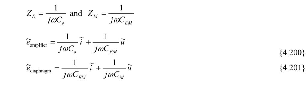
Note that this set of equations is not typical of the transfer functions used in this analysis. There are two inputs and two outputs. Often a matrix approach is used for multiple input, multiple out equations.

Since bond graphs are not unique, one based on Beranek’s models ([9], page 73 Figure 3.37) for electrostatic transducers can be used, and then it will be shown that it satisfies {4.202}.
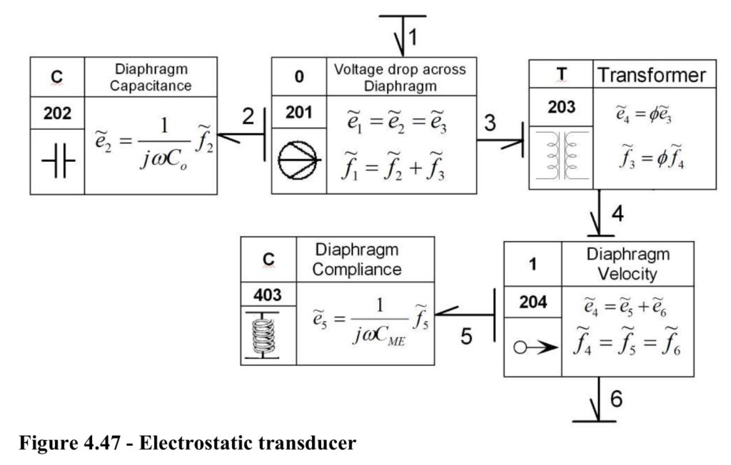
The new parameters in Figure 4.47 are:
The transformer modulus, ϕ, defined as

and the effective Diaphragm Compliance. CME in C403, defined as

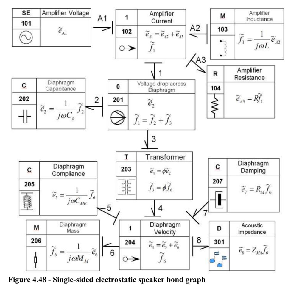
Figure 4.48 shows the complete bond graph for the single sided electrostatic speaker shown in Figure 4.46. Let
The negative sign on
is used because
bond 6 shows the flow as an output.
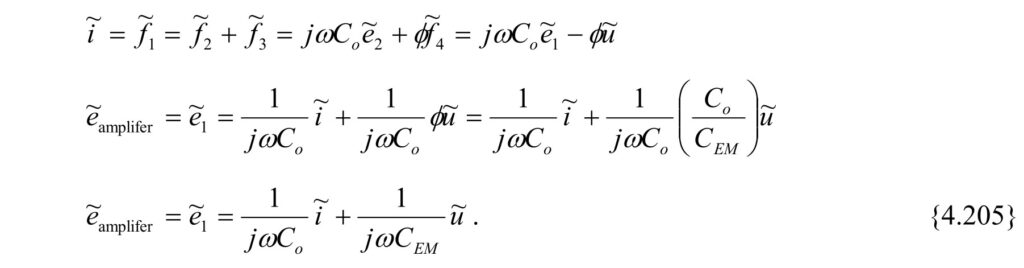
At the electrical terminal, bond 1,
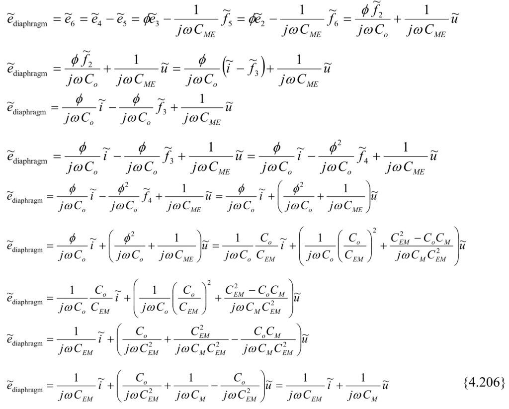
At the mechanical terminal, bond 6,
The basic device shown in Figure 4.47 represents other field coupled transducers such as condenser microphones and piezo-ceramic transducers. The performance characteristics of the device will be discussed in later sections on microphones.
Double-sided Electrostatic Speaker
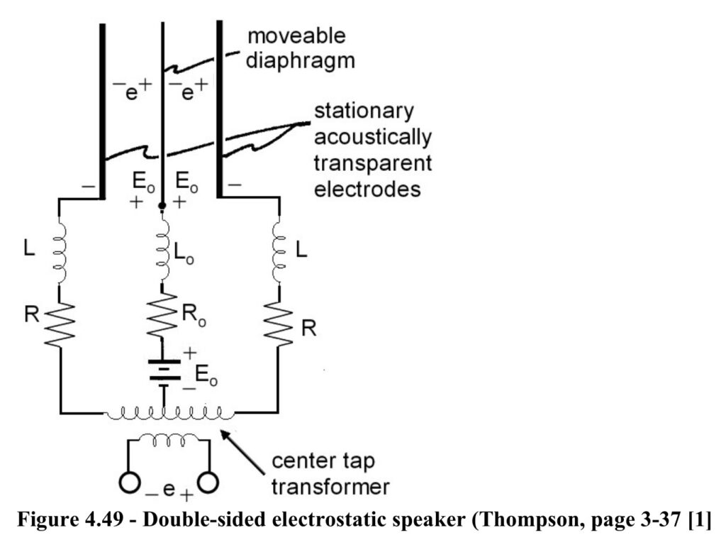
The double-sided electrostatic speaker shown in Figure 4.49 can be modeled using the bond graph in Figure 4.46. With this arrangement xo =0 is independent of Eo.. The device is more linear than a one-sided electrostatic speaker. Modern versions use curved diaphragms and can cover a wide frequency range 50 Hz to 20,000 Hz.
Microphones
The acoustic source transducers analyzed here are reciprocal devices. They may also be used as receivers. They have the same directivity pattern in either mode of operation – the ratio of the transmitting response to the receiving response, with the same electrical termination, is known as the reciprocity constant.
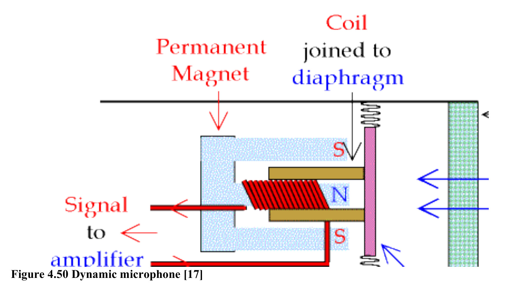
The dynamic microphone shown in Figure 4.50 has a small movable induction coil attached to a diaphragm. The induction coil is positioned in the magnetic field of a permanent magnet. When the diaphragm vibrates, the coil moves in the magnetic field, producing a varying current in the coil. Dynamic microphones use magnetic elements in a manner that is basically the reverse of that used by loudspeakers to convert electrical energy into sound. Dynamic microphones are rugged, reliable, and relatively inexpensive, and are used in a wide variety of applications.
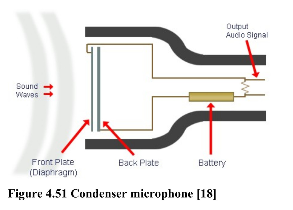
The reciprocal of an electrostatic loudspeaker is a condenser microphone. An example is shown in Figure 4.51. A capacitor has two plates with a voltage between them. In the condenser microphone, one of these plates is made of light material and acts as the diaphragm. The diaphragm vibrates when struck by sound waves, changing the distance between the two plates and therefore changing the capacitance. When the plates are closer together, capacitance increases and a charge current occurs. When the plates are further apart, capacitance decreases and a discharge current occurs. A voltage is required across the capacitor. This voltage is often provided by an external power supply but can be supplied by a battery in the microphone.
Expensive hiqh quality condenser microphones are used in laboratory and studio recording applications.
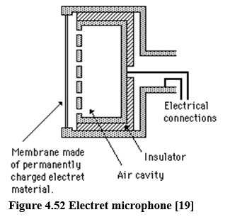
A variation on the condenser microphone is the electret type shown in Figure 4.52. An electret is a dielectric plastic material that has been “permanently” electrically charged. Electret microphones have now become the most common type of all, used in many applications including cellular phones. Unlike other condenser microphones they require no polarizing voltage. Overtime the electret plastic can lose its charge and stop working.
Other types of microphones include:
- Ribbon microphones with a corrugated metal ribbon suspended in a magnetic field
- Carbon microphones are non-reciprocal devices with carbon granules pressed between two metal plates. A voltage is applied across the metal plates, causing a current to flow through the carbon. One of the plates, the diaphragm, is exposed to the incident sound applying a varying pressure to the carbon. The changing pressure deforms the granules, causing the contact area between each pair of adjacent granules to change, and this causes the electrical resistance and hence the current to vary.
- Piezo microphones use crystals that produce a voltage when subjected to pressure.
If only one side of the diaphragm is exposed to sound, the microphone output depends on sound pressure. Pressure microphones are omnidirectional for low to medium frequency sound.
If both sides of the diaphragm are exposed to the sound, the voltage generated by the diaphragm depends on the difference of the pressure in front and behind the diaphragm. Pressure gradient microphones are bidirectional.
Making a device incorporating both pressure and pressure gradient response gives one-sided directional response and are given names such as a cardioid microphone.
The analog circuits developed in earlier sections for the moving coil and electrostatic loudspeakers are valid for microphones except now the excitation is applied at the mechanical terminals and the output is at the electrical terminals.
Recall the generic model for an acoustic receiver shown in Figure 3.1. One new concept that is needed is a way to model a radiation signal modulating a power. Thevenin’s Theorem is the approach used to provide the appropriate interface between the incoming signal and the power modulation.
Thevenin’s Theorem
Thevenin’s theorem is most often expressed in electric circuit terminology, so let’s first review it in the electric domain, and then extend it to the general case.
Thevenin’s theorem states that any two terminal linear network is equivalent to an ideal voltage source, E, in series with an impedance, Z. E is the open-circuit voltage across the 2 terminals and Z is the impedance measured at the terminals when all sources within the network are replaced by their internal impedances (zero for a voltage source).
Figure 4.53 shows an electrical circuit and its bond graph that is used as an example.
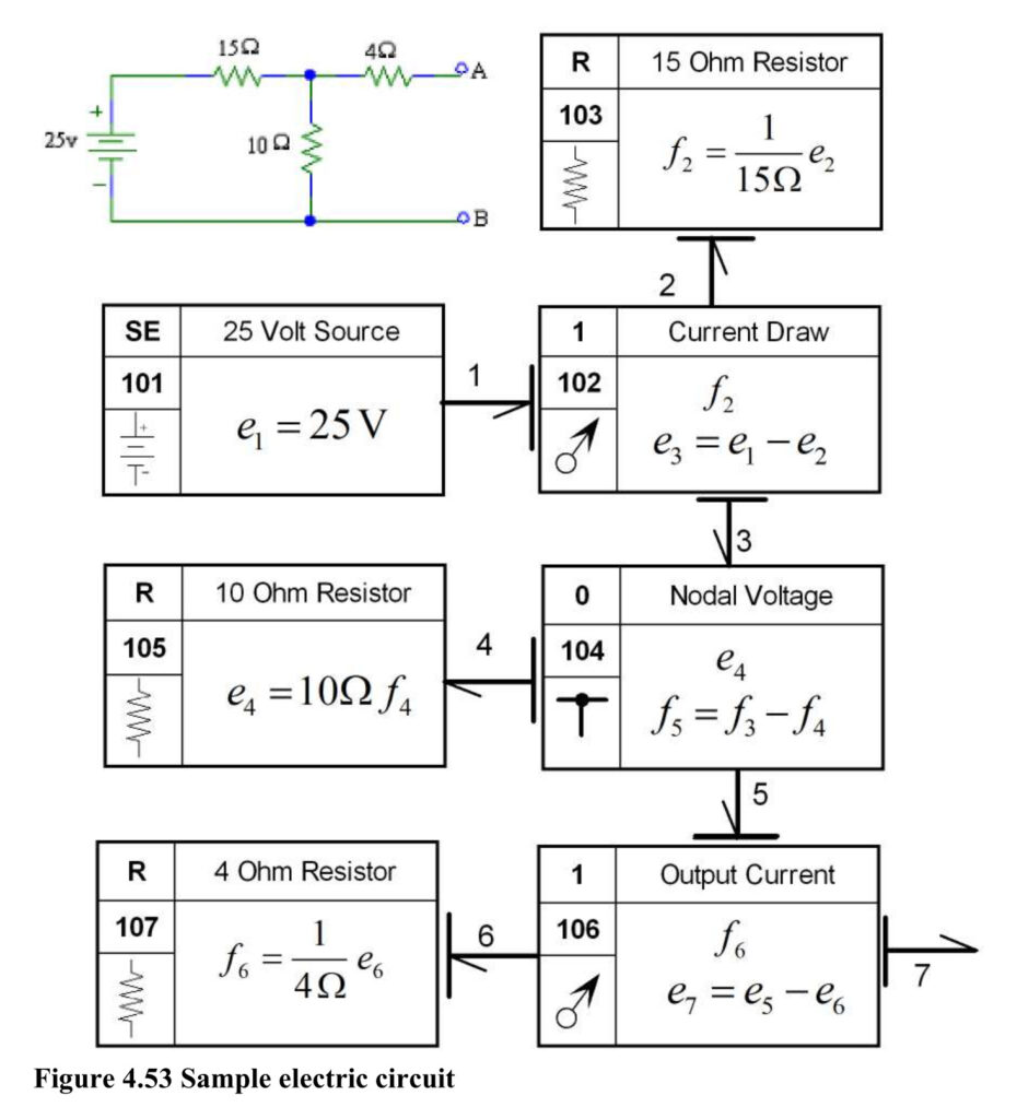
To find the Thevenin Equivalent Circuit for Figure 4.53, the open circuit voltage across terminals A and B, and the equivalent impedance are needed. These are determined using the following steps.
Step 1: | Find Thevenin’s Voltage (the open circuit voltage between terminals A and B): |
| Because the terminals are open, there will be no current flowing through the 4W resistor,(f5=f6=f7=0) and therefore, no voltage drop across it, e6=0. So, e7, the open circuit voltage (VTH) equals e5=e4, the voltage across the 10W resistor. From 1102, and 0104, e4=e3=e1-e. 25 = 15f2+10f4=25f1.So f1= 1 Amp, and e7 = VTH = 10v. |
| Step 2: | Find Thevenin’s Resistance (the resistance seen looking into terminals A and B): |
| First, replace the voltage source with its Ideal Internal Resistance . A voltage source internal resistance is zero so the circuit with attached Ohm meter is given in Figure 4.54. |
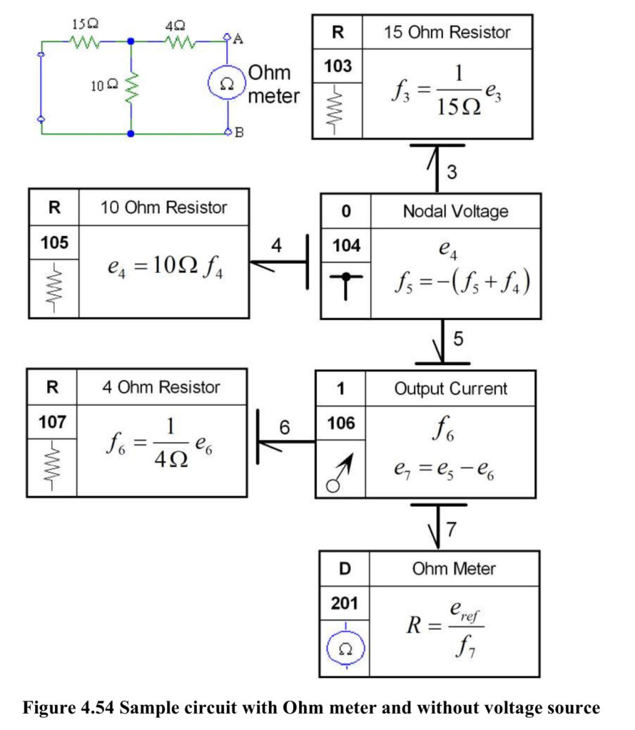
Figure 4.54 Sample circuit with Ohm meter and without voltage source
| In this circuit, the ohmmeter would measure 10 ohms (the 4 ohm resistor is in series with the parallel combination of the 10 ohm and 15 ohm resistors). | |
| Step 3: | Draw the Thevenin Equivalent Circuit (shown in Figure 4.55): |
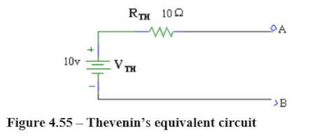
Generalized Thevenin’s Theorem
By replacing the electrical domain terminology in Thevenin’s Theorem with generalized bond graph terminology a form useful for modeling an acoustic source is obtained.
Any 1-port linear network is equivalent, at its port, to an ideal effort source, e, in series with an impedance Z where, e, is the effort at the port when the flow at the port is zero, and Z is the impedance measured at the port when all sources within the network are replaced by their internal impedances (zero for an effort source and infinity for a flow source).
For a receiver in an acoustic field, a division of the system into two networks can be realized by separating the device at the bond between the transducer’s active face and the acoustic medium as shown in Figure 4.56.
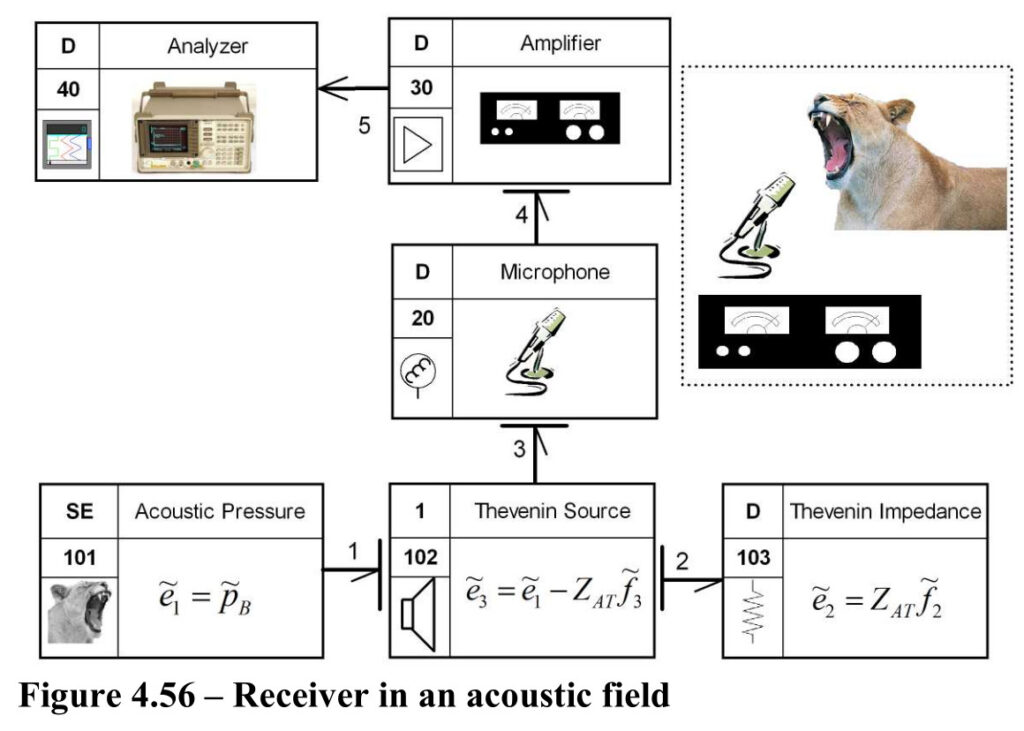
Element SE101 is a modulated pressure source. The signal controlling SE101 is not shown. With the average pressure over the blocked active surface, (area = S) of the transducer. Blocked means that the diaphragm is constrained to not move, thus when the value for is calculated. ZAT is the acoustic radiation impedance on the active surface.
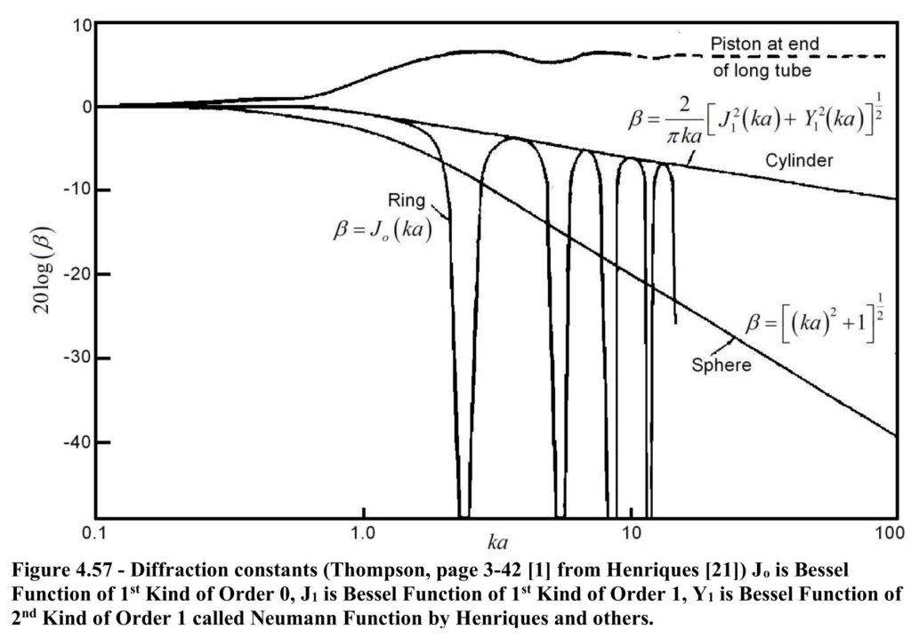
The blocked pressure, is related to the free field pressure, by the diffraction constant,

The diffraction value depends on the sound wavelength compared to the size of the microphone, (i.e. it is a function of frequency). If the sound wavelength is much greater than the receiver,
Bobber [20] gives a general expression that relates the diffraction constant, to the directivity,

For a baffled circular piston

where a is the radius of the piston, and J1 is a Bessel Function. The directivity function for a baffled circular piston is

Therefore for a baffled circular piston

Equation {4.211} is true for any baffled piston regardless of shape or size, thus from {4.208}

giving

.

Figure 4.57 shows the diffraction constants for several other shapes of receivers.
Receiving response of moving coil (electrodynamic) microphone
Consider a dynamic microphone as shown in Figure 4.50 attached to a pre-amp. Setting the input impedance of the pre-amp to infinity allows signal analysis (rather than power analysis) to be performed with any devices downstream from the transducer. Figure 4.58 shows the bond graph of the receiving system formulated by converting the loudspeaker model shown in Figure 4.6 a receiving model.
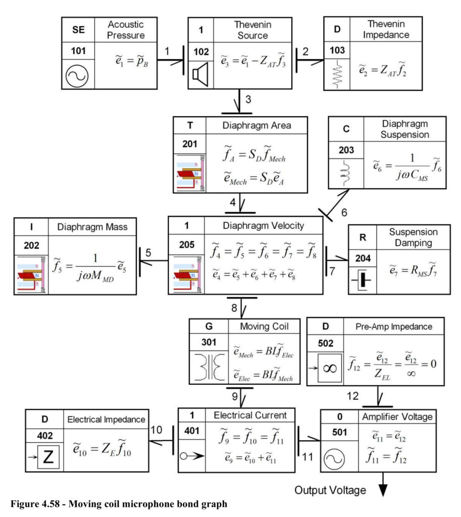
Note that D502 with (ZEL = infinity) makes the electrical terminals effectively open circuited since and
bond 8 becomes a signal indicating the Diaphragm Velocity and G301 can be treated as an Analog Block.
Following the procedure used to reduce Figure 4.6 to Figure 4.8. Figure 4.58 is simplified to give Figure 4.59.
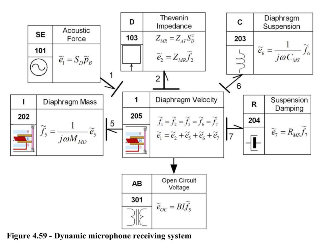
Expanding the effort equation of Element 1205 in Figure 4.59 gives


Then from AB301

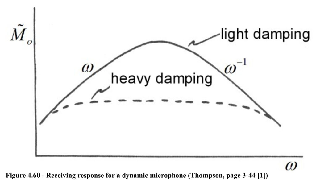
The receiving response, can be shown to be

At low frequency, the compliance term is dominant giving

Above the resonance frequency, the mass term dominants giving

The above indicates that a dynamic microphone does not have a flat response curve. However, making RM large flattens the response as shown by the dashed line in Figure 4.60.
Receiving response of condenser and electrostatic microphones
Conceptual drawings of electrostatic, condenser/capacitor and electret microphones were shown in Figures 4.51, and 4.52. Like the approach used for the dynamic microphone, the electrostatic speaker model shown in Figure 4.48 can be converted to the receiving model shown in Figure 4.61.
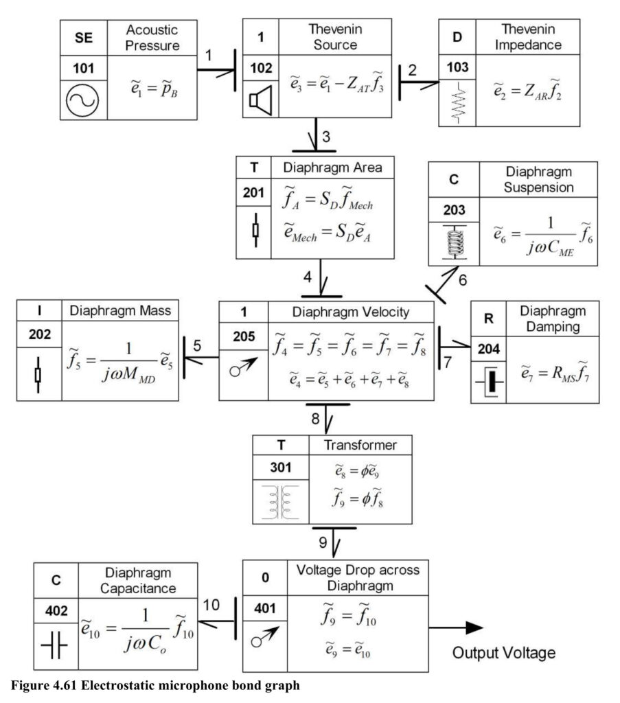
Recall from {4.203} and {4.204} that the transformer modulus, ϕ, is defined as

and the effective Diaphragm Compliance. CME in C203, is defined as

The parameters of electrostatic microphones are selected so the operating frequency range is below the natural frequency of the device, i.e. the behavior is compliance controlled. In the range below the natural frequency, Figure 4.61 simplifies to Figure 4.62.
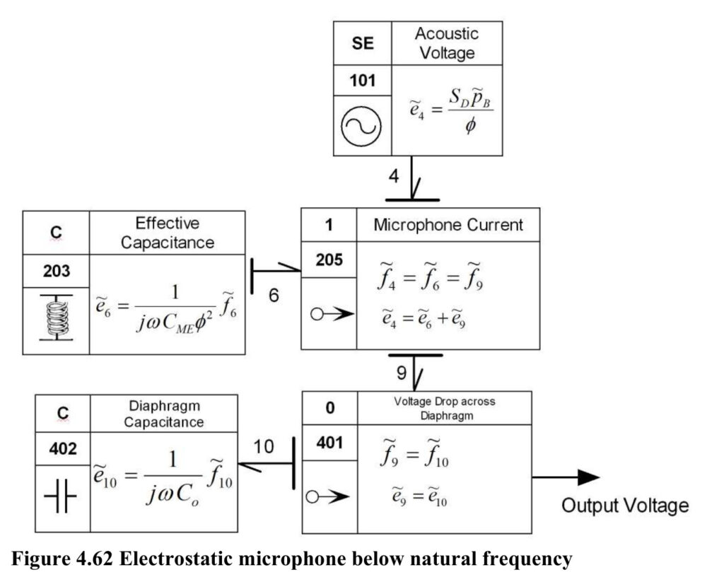
The solution approach used earlier can be applied to the equations in Figure 4.62 to determine the output voltage. From element 1205,



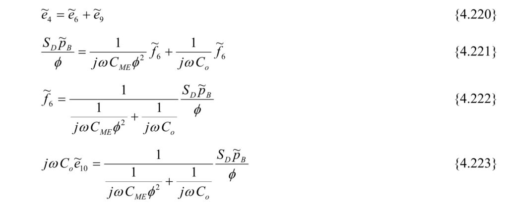

Equation {4.224} shows that below the resonance frequency the ratio of the output voltage to the sound pressure is a constant given by

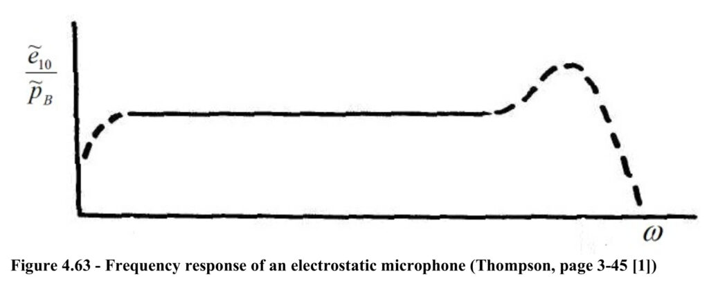
Figure 4.63 conceptually shows the frequency response for a condenser microphone. The resonance frequency can be placed outside the range of interest. For example, a high quality ½ inch microphone has a flat response from 10 Hz to 40 kHz.
####