Chapter 2 – Acoustic Elements – Analysis of Audio Transducers

Acoustic Elements

Electro-acoustic transducers contain electrical, mechanical and acoustic devices. The bond graph elements for electrical and mechanical characteristics are straight forward, and can be found in references such as [3, 4]. Unfortunately, the same simplicity is not available for acoustic elements.

Lumped parameter models are good approximations to behavior of continuous media when the dimensions of the device are small compared to the wavelength of the vibration.

In a non-dispersive media, wavelength, λ, wave speed, c, and frequency, f, are related by:

\lambda\,[\mathrm{m}] = \frac{c\,[\mathrm{m/s}]}{f\,[\mathrm{Hz}]}

{2.1}

(When equations show text within brackets that indicates typical units for those variables.)

Thompson [1] states that a good definition for dimensions that are small compared to wavelength is:

L < \frac{\lambda}{16}

{2.2}

then put {2.2} into {2.1} and use algebra to give

f < \frac{c}{16L}\,[\mathrm{Hz}]

{2.3}

Figure 2.1 shows characteristic length limit vs frequency for lumped parameter acoustic models involving air at room temperature.

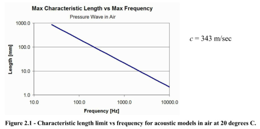
Since the wave speed for electromagnetic phenomena is close to the speed of light in a vacuum, electric circuit models based on lumped parameters are valid for all acoustic frequencies (20-20,000 Hz).

There are three types of fundamental acoustic elements:

Acoustic compliance stores potential energy
Acoustic mass stores kinetic energy
Acoustic resistance dissipates energy either by converting mechanical vibration into heat, or radiating acoustic waves.

When considering a general device, these three characteristics can be combined and referred to as acoustic impedance.

Acoustic Impedance

Reference [1] gives the derivation of the general acoustic wave equation. Considering steady state one-dimensional situations, the general acoustic wave equation reduces to the one-dimensional Helmholtz equation [7]

\frac{d^2 p}{dx^2} + k^2 p = 0

{2.4}

where k, the wave number, is an alternative way of specifying frequency

k = \frac{2\pi}{\lambda} = \frac{2\pi f}{c} = \frac{\omega}{c}.

{2.5}

If you had a course on differential equations, you will recognize the solution of {2.4} is

p(x) = A\sin(kx) + B\cos(kx)

{2.6}

then by taking the partial derivative of p with respect to x

\frac{\partial p}{\partial x} = kA\cos(kx) – kB\sin(kx)

{2.7}

Now we are ready to develop equation for plane waves propagating in long tubes.

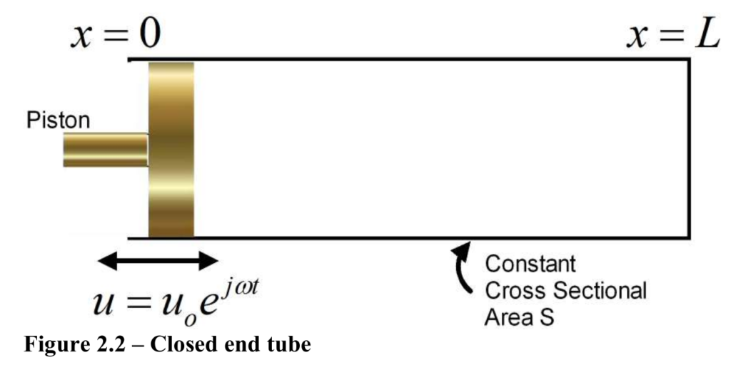
Consider a constant cross-sectional area tube whose lateral dimensions are small compared to the length L. A piston at one end causes plane waves to propagate to and fro in the tube. A constant amplitude of the piston moving in a sinusoidal motion at x = 0 can be represented as:

u = u_0 e^{j\omega t}

Recall that Euler’s identity between the complex exponential function and trigonometric functions gives

e^{j\omega t} = \cos(\omega t) + j\sin(\omega t)

{2.8}

Since the Helmholtz equation is being used, the time varying part can be ignored and the boundary condition at the piston is

u = u_0

{2.9}

Doing this simplifies the algebra. If the time variation is needed,

e^{j\omega t}

can be put back in the developed equations. Many people call u_o velocity. It is more appropriate to call it velocity amplitude.

The quantity u_o can be a complex number, but usually it is set to a real number, then it is the magnitude of the input velocity amplitude, |u₀|.

Figure 2.2 shows a tube with a closed end. Figure 2.3 shows a tube with an open end.

Euler’s equation of motion[2.1] gives the relationship between the particle velocity, density, and pressure at a point in a fluid:

u(x) = -\frac{1}{j\,\omega\,\rho_0}\,\frac{\partial p}{\partial x}

{2.10}

Substituting {2.5} and {2.7} into {2.10} gives

u(x) = -\frac{1}{j\,\omega\,\rho_0}\,k(A\cos(kx)-B\sin(kx)) =

-\frac{j*j}{j*\omega\,\rho_0}\,\frac{\omega}{c}(A\cos(kx)-B\sin(kx))

since

j^2 = -1

The above equation simplifies to:

u(x) = \frac{j}{\rho_0}{c}\,(A\cos(kx)-B\sin(kx))

{2.11}

Coefficients A and B are determined by applying the boundary conditions.

At the piston end, x = 0, since cos(0) = 1, and sin(0) = 0

u(x=0) = u_0 = \frac{j}{\rho_0}(A\cos(0) – B\sin(0)) = \frac{jA}{\rho_0}

{2.12}

therefore

A = \frac{\rho_0}{j} = -\,j\,\rho_0\,c\,u_0

{2.13}

Notice that A is independent of the boundary condition on the right end of the tube. The boundary condition on the right end is used to solve for coefficient B.

For a closed end tube, the velocity at the right end must be zero. Substituting {2.11} into {2.10} gives

therefore recalling that cot/sin = cot

Substituting {2.13} and {2.16} into {2.6} gives the relationship between pressure amplitude and the magnitude of particle velocity amplitude for a closed end tube

Therefore at the piston, x=0

In the acoustic domain, the effort variable is pressure, and the flow variable is volume velocity, U.

The volume velocity for a plane wave in a tube is

U = uS. {2.19}

u is the piston axial velocity and S is the cross-sectional area of the piston. Equation {2.18} can be written to provide a relationship between input pressure and volume velocity

The acoustic impedance at a point is the ratio of the acoustic pressure to the volume velocity. Hence the input acoustic impedance for a closed tube is:

Using the Laurent Expansion for the cotangent, for small kL

giving

Taking just the first term of the Laurent Expansion gives

Since volume of the tube is given by V =SL and using the definition for k, {2.5} the equation {2.24} can be written as

Then introducing

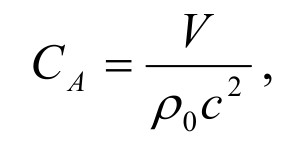
{2.25} can be rewritten as

This equation is the same form as the impedance for a spring [2.2]. Thus C_A is called acoustic compliance.

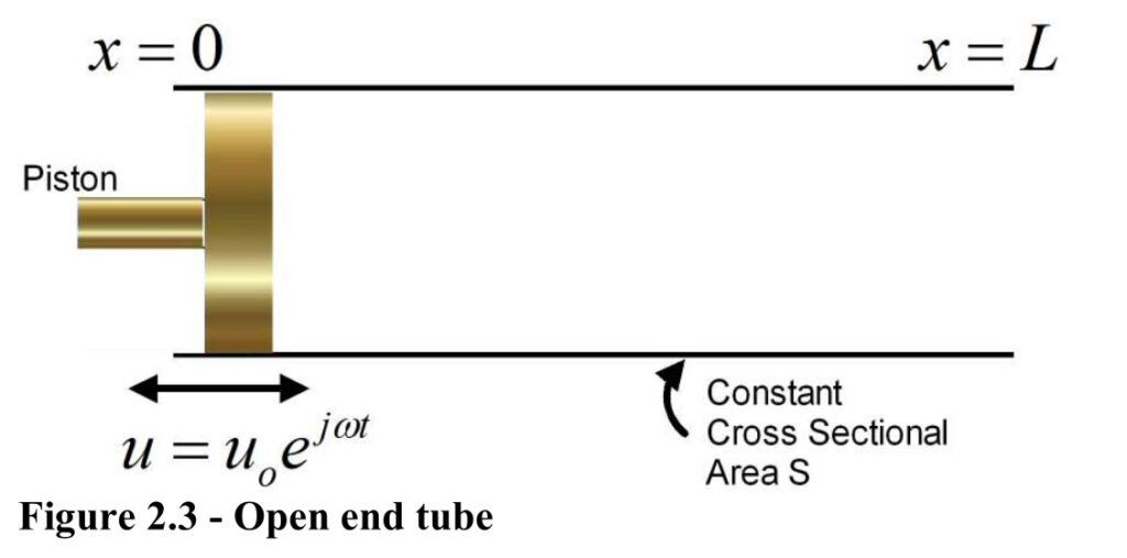
Consider now, the open end tube shown in Figure 2.3. Assume that negligible sound is radiated from the open end. For this to be true, the pressure at x = L must be zero. Using this boundary condition, equation {2.6} becomes

Since {2.13} defines A whether the tube is open or closed,

Substituting {2.27} and {2.13} into {2.6} gives the relationship between pressure amplitude and the magnitude of particle velocity amplitude for an open end tube

At the piston, x = 0,

Hence the input acoustic impedance (Z_A at x=0) is

The Taylor Expansion of tan(kL), for small kL is

When

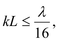
only the first term of {2,31} is needed to

approximate the tangent, giving

The quantity

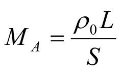
is called the acoustic mass.

Recall equation {2.23} holds when

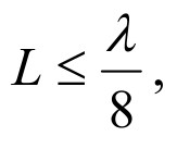
but we can use

when

\frac{\lambda}{16} < L \le \frac{\lambda}{8}.

Equation {2.33} indicates that a closed tube

with

\frac{\lambda}{16} < L \le \frac{\lambda}{8}

behaves as a series combination of a spring

and a mass.

Acoustic Mass

The boundary condition used to define the acoustic mass, {2.32}, is too restrictive. If the pressure is not zero at the end, then air will be accelerated beyond the length of the tube. This extra length is noted by considering L’, the effective length of the tube, where

L’ = L + “end corrections”.

The pressure – volume velocity relationship then is:

where

and p is the pressure differential from one end to the other. U is the volume velocity of the acoustic wave in the tube. End corrections for flanged and unflanged tubes can be found in Reference [7].

Acoustic Compliance

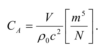
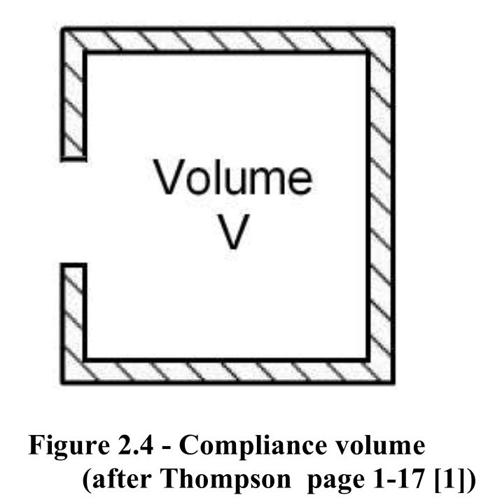
Although {2.26} was developed for a closed tube with a piston, the acoustic compliance element holds for any closed rigid walled container with all dimensions small compared to the wavelength (conceptually shown in Figure 2.4). With pressure p acting to compress the volume V, and U the volume velocity flowing into V,

where

Acoustic Resistance

Acoustic resistance, R_A, accounts for energy converted to heat or energy acoustically radiated. Acoustic resistance is the analogue of mechanical resistance, R_M.

For a mechanical damper the effort – flow relationship is:

with E_M = force, and F_M = translational velocity. The pressure – volume velocity relationship then is:

with E_A = pressure, F_A = volume velocity and

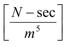
is called SI acoustic ohms.

Mixed Mass-Compliance

A cavity with holes on opposite ends, shown in Figure 2.5, is an example of a mixed mass-compliance element. Figure 2.6 is a bond graph for this device, when connected to effort sources at each face.

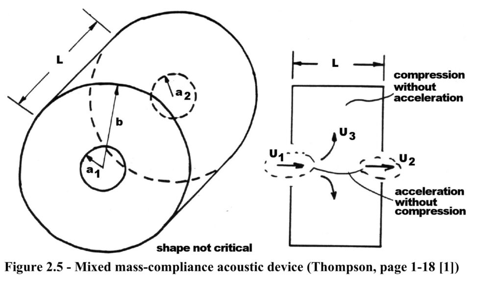
As a review for using annotated bond graphs, the following will walk through how to get from the device shown in Figure 2.5 to its completed bond graph in Figure 2.6.

Starting from left to right the first block represents the input pressure.

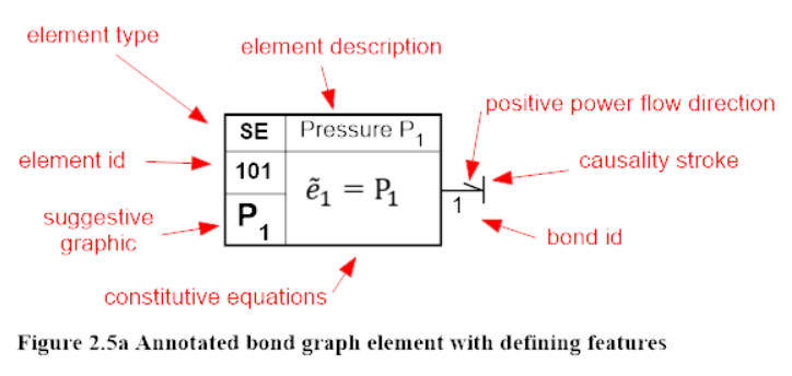
Figure 2.5a shows an effort source which is indicated with the element type shown in the top left corner. The top right box is text used to describe the element (element description). The middle box on the left side is reserved for a unique arbitrary integer used to identify the element (element id). Below it is a graphic used to indicate what the element represents (suggestive graphic). The remaining box contains the constitutive equations for the element. Since an effort source strength is independent of the flow strength, for an effort source there is no need to indicate its flow. Since element 101 is an effort source that determines the type of causality, the bond between element 101 and 200 (shown in Figure 2.5b) has the causality stroke at the arrowhead. The direction of the arrow is also arbitrary and indicates the positive effort direction. Each bond connects two elements. The formal name for the effort and flow variables on a bond is defined by the element identifiers, but to make the constitutive equations shorter, the bonds are given integer values (bond Id) which can be considered a nickname.

Figure 2.5b shows element 101 shown in Figure 2.5a and element 200.

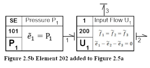
Element 200 is a multi-port element with all ports having the same flow strength. By convention these types of elements are called 1-elements. 1-elements can have only one bond with flow causality. In this case it is bond 3. Since power is conserved in 1-elements the sum of the efforts in the bonds accompanying element 200 sum to zero. The arrows show that bond 1 flows into element 200, and bonds 2 and 3 flow out of element 200. Thus as show in Figure 2.5b

\tilde f_1=\tilde f_2=\tilde f_3

\tilde e_1-\tilde e_2-\tilde e_3=0

The tilde is applied to effort and flow variables to indicate that they could vary from measured values since approximations for trigonometric functions have been used, and the equations have been derived using lumped parameters.

In Figure 2.5c elements 201 and 300 are added.

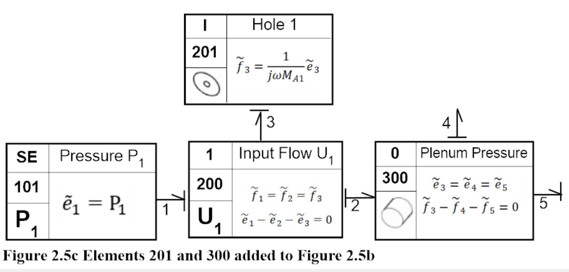
Thompson[1] explains that the hole acts as an acoustic mass and is thus an inertia element with element type I, and an inertial constitutive relationship. The constitutive relation shown in Equation 2.32 can be rewritten as

\tilde f_3 = \frac {1} {j\omega M_{A1}} \tilde e_3

Element 300 is multi-port element with all ports having the same effort. By convention it is call a 0-element. 0-elements can have only one bond with effort causality. In this case it is bond 4. Since power is conserved in 0-elements, the sum of the flows in the bonds accompanying element 300 sum to zero. The arrows show that bond 2 flows into element 300, and bonds 4 and 5 flow out of element 300. Thus, as show in Figure 2.5c

\tilde e_2=\tilde e_4=\tilde e_5

\tilde f_2-\tilde f_4-\tilde f_5=0

Elements 301 and 400 are added to Figure 2.5c to give Figure 2.5d.

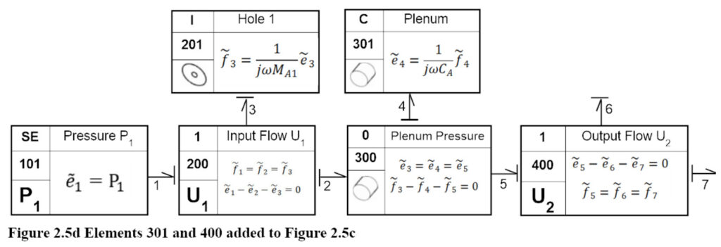
The Plenum as explained by Thompson[1] behaves as an acoustic compliance element and thus element 301 has element type C and a compliance constitutive equation

\tilde e_4 = \frac {1} {j\omega C_{A}} \tilde f_4

Element 400 is similar to Element 200 and shows that the efforts of all its bonds sum to zero, and the flows of all its bonds are equal.

Elements 401 and 402 are added to Figure 2.5d to complete the bond graph shown in Figure 2.6

Similiar to the elements shown in Figure 2.5d, Element 401 is an inertia element and element 402 is an effort source.

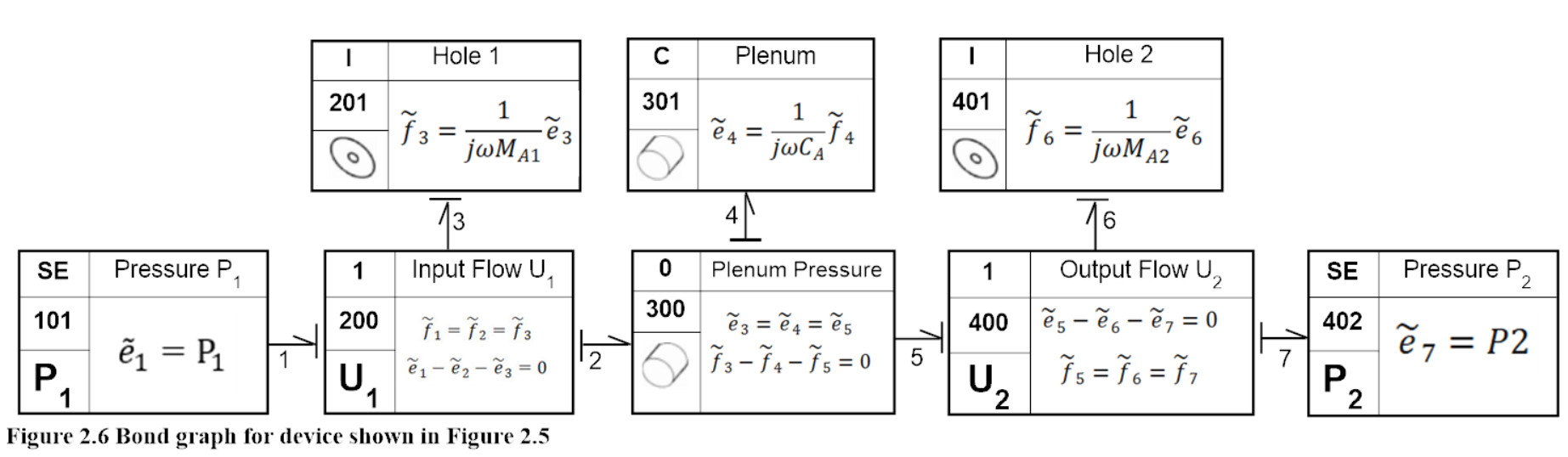
Figure 2.6 – Bond graph for device shown in Figure 2.5

According to Thompson[1], simple formulae for the values of M_A1, M_A2, and C_A as functions of a₁, a₂, b, and L are not available.

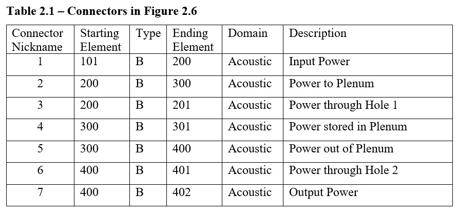
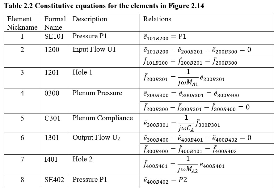
The information contained in bond graphs can also be specified in tables. Table 2.1 lists the connectors in Figure 2.6, and Table 2.2 lists the connectors. In Chapter 4, such tables will be used to help the discussion leading to determine the frequency response of various audio transducers.

Helmholtz Resonator

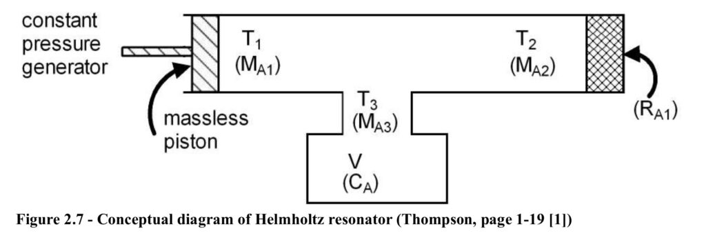
A bond graph model of a Helmholtz Resonator (Figure 2.7) will now be developed to demonstrate how a collection of fundamental acoustic elements is used to analyze the behavior of an acoustic device.

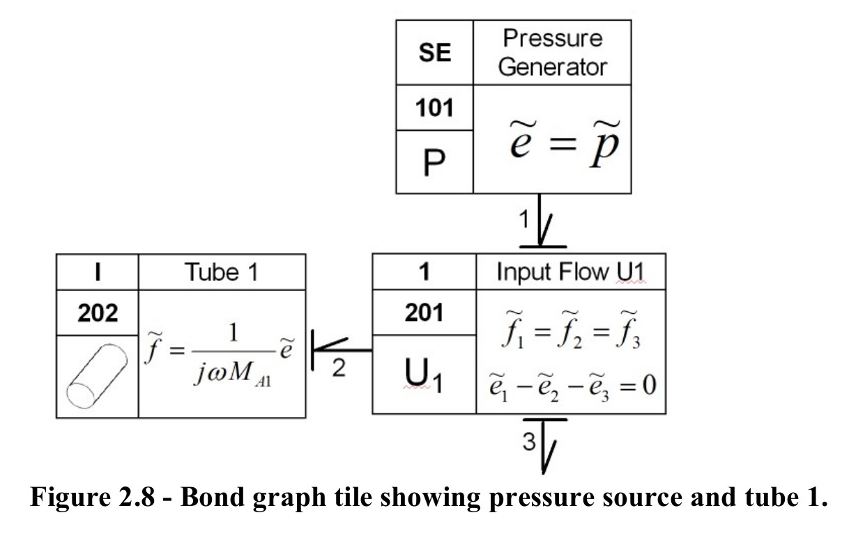
First, select elements for each feature in the system. Referring to the bond graph tile in Figure 2.8, the constant pressure source is an effort source (SE101). Tube 1, T₁ in Figure 2.7, is an acoustic mass (I202). The two elements see the same flow, so are connected by a 1-junction (1201). The standard bonds on I202 and SE101, determine the causality of the third bond on 1201.

The output from Tube 1 connects at a junction with Tube 2 and Tube 3. At the connection point all three tubes see the same pressure, so it is represented by a 0-Junction shown in Figure 2.9.

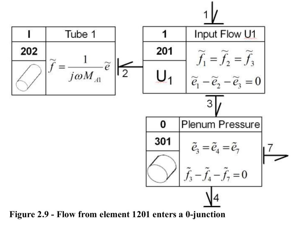
All the flow through Tube 2 (acoustic mass, I402) goes through the acoustic resistance, R403, and leaves the system at effort source SE501. The standard causality for I402 defines all the causalities of the bonds connected to 1401. These elements are shown in Figure 2.10.

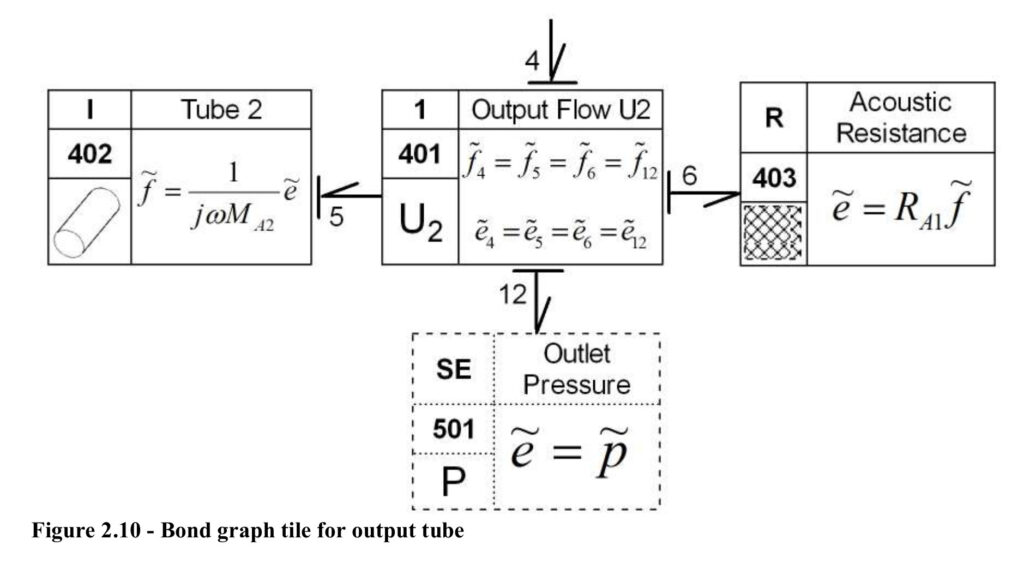
Element SE501 is shown with phantom lines, because the pressure of the atmosphere is considered “ground”, that is it remains at 0 gage pressure irrespective of the flow. Since no power flows to grounded elements, there is usually no need to explicitly show them in bond graphs. Grounded elements that could be shown in the remaining figures are omitted.

Since 201B301 contacts element 0301 as a causal flow, and 301B401 contacts element 0301 as a causal flow, there must be another bond that contacts element 0301 as a causal effort. This relationship allows the above bond graph tiles to be connected giving Figure 2.11.

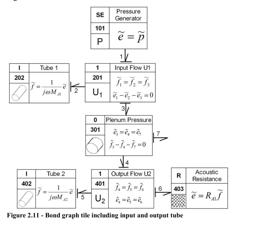
The as yet undefined bond on 301 leaves 301 with flow causality. This flow goes through Tube 3 into Volume V. As a lumped parameter, the mass in Tube 3 acts as a slug of incompressible air – both ends of the tube have the same volume velocity. Thus Tube 3 and Volume V see the same flow, so they connect with a 1-junction, 1302 shown in Figure 2.12. Since 301B302 enters 1302 with flow causality that requires that all the other bonds on 1302 enter 1302 with effort causality. Using the standard causality, an acoustic mass cannot be directly connected to 1302. This means that a 0-Junction, 0305, must be added between 1302 and I303, and Tube 3 will not be modeled as a pure mass. Figure 2.12 gives the bond graph tile developed so far.

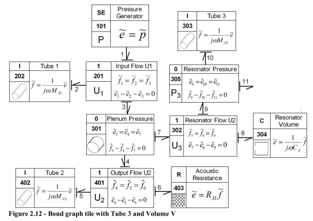
An element is needed to define the pressure of Junction 0305, but the concept model doesn’t have any more elements. A phantom element 306 with effort causality entering 0305 is added. Element 306 could be either an acoustic resistance or an acoustic compliance. For convenience, assume there are viscous flow losses in Tube 3, so an acoustic resistance is added to get the completed bond graph shown in Figure 2.13.

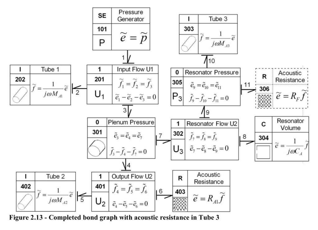
Figure 2.13 indicates that to solve the system equations in the time domain a non-zero flow resistance is needed in Tube 3. However, since the system equations will be solved in the frequency domain, the acoustic resistance parameter in R306, R_F_,can be set to zero. That action will force F_305B303 to equal F_302B305, and therefore elements 0305 and R306 can be removed to give Figure 2.14.

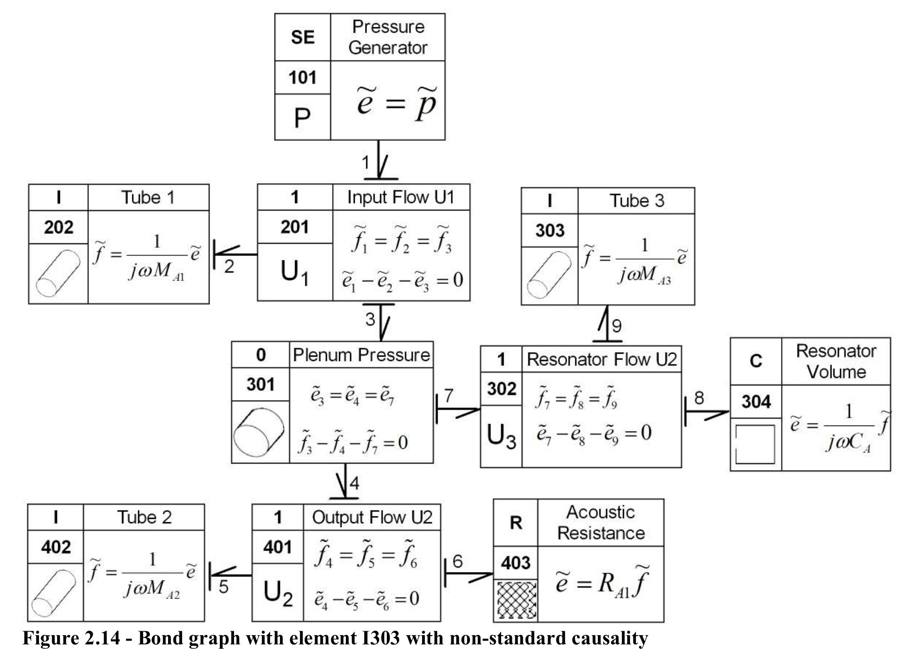
A list describing each connector in Figure 2.14 is given in Table 2.3

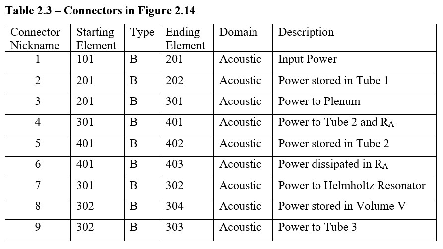
Table 2.4 is constructed from the information in Figure 2.14

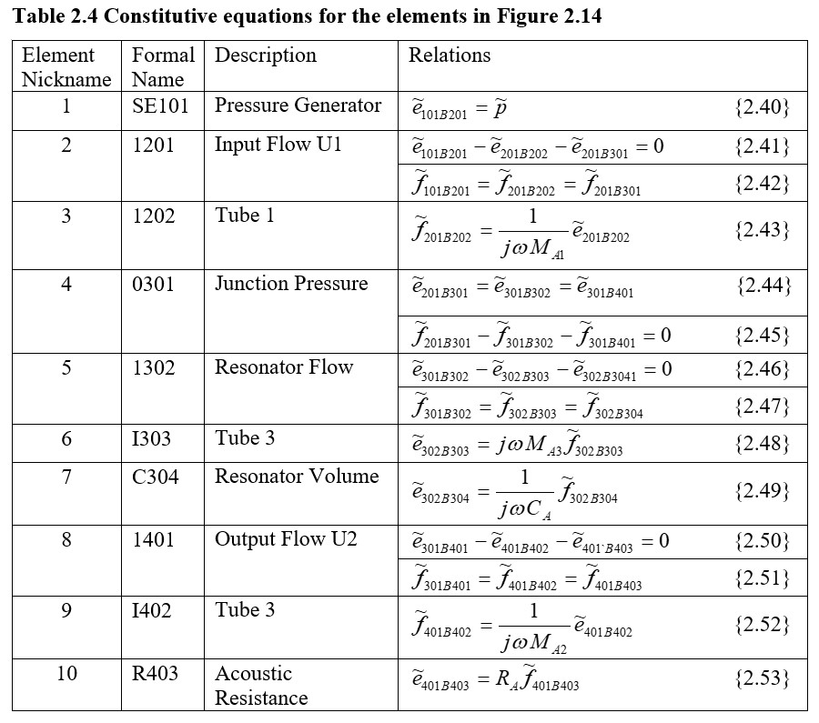
A Helmholtz resonator is used to minimize the absolute value of the output flow. The equations in Table 2.4 could be used to determine the conditions necessary to minimize

U_2 = \tilde{f}_{301B401},

however, a benefit of bond graphs is that they can provide insight so it may be unnecessary to solve all the equations.

An absolute minimum for U₂, is U₂= 0. Assume U₂= 0 and then determine the implications of this assumption.

From {2.45},

with

\tilde{f}_{301B401} =0,

For this to be true, then element 1302 can provide no flow resistance therefore

Substituting {2.48} and {2.49) into {2.56} gives

Solving {2.57} gives

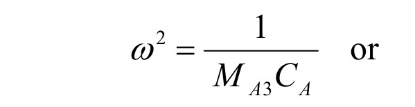
Equation {2.58} is the familiar relationship for the resonance frequency for an oscillator with mass M_A3 and compliance C_A. Equation {2.58} specifies the product of the acoustic mass and the acoustic compliance to minimize the output.

Mechanical – Acoustic Transformer

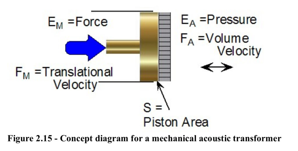
An ideal piston, with cross-sectional area S, is a transformer between the translational mechanical domain and the acoustic domain.

S, the piston area, is called the transformer modulus. Multiplying {2.59} and {2.60} shows that power is conserved.

Power

There are several common measures of power

Instantaneous power
Average power
Complex power

Referring to the phasor diagram in Figure 2.16, peak quantities (not RMS) of the flow and effort variables are:

with

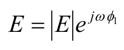
and

with

F=|E|e^{j\omega \phi_2}

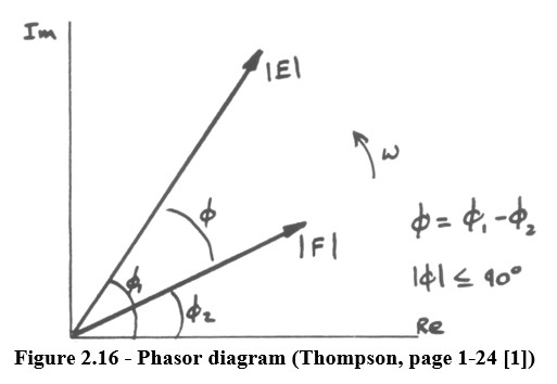
Instantaneous power is the product of E(t) and F(t)

P_{inst}=EF=|E||F|cos(\omega t+\phi_1)cos(\omega t+\phi_2)

The average power is determined from the instantaneous power using

since

The complex power is one half the complex conjugate (indicated by an asterisk) of effort times flow, or equivalently one half the effort times the complex conjugate of the flow.

With

This quantity is always >0, and has units of watts. It is called the active power and represents the radiated acoustic energy flow.

Q_ave is the power that is oscillating between the source and the load. It is called the reactive power.

Flow, F, is related to effort, E, and the complex impedance, Z, using the generalized form of Ohm’s Law.

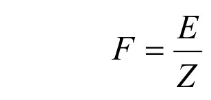
where F, E, Z are all complex.

Then, complex power, P_complex , is

and similarly

The phase angle is related to the complex impedance by:

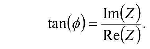
In this chapter acoustic plane wave elements were introduced. In the next chapter summary material on spherical acoustic waves is provided.