In Chapter 2 the approach for modeling acoustic interactions with electro-mechanical devices was introduced by considering plane waves. The behavior of spherical acoustic waves is also important, especially for understanding radiation from a transducer.
References [7] and [8] cover this material in detail. This chapter is provided to highlight those topics that will be used to evaluate audio transducers.
Modeling Radiating Systems
Radiation is a process that uses waves to transfer energy from one part of a system to another. Radiation can also pass through a system boundary, and thus add or remove energy. Figure 3.1 shows a conceptual model for an acoustic receiver. Figure 3.2 shows a corresponding model for an acoustic transmitter.
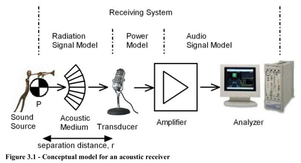
Both models have similar components, so for convenience consider the acoustic transmitter model in Figure 3.2
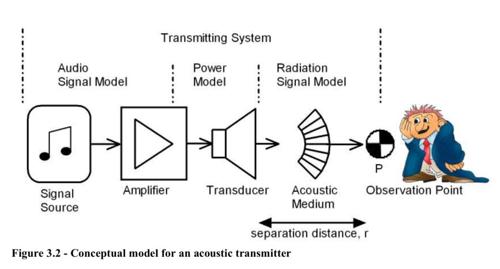
The signal source provides information to the amplifier. For modeling purposes part of the amplifier is considered a signal processor, and the other part provides modulated power to the transducer. The connection between the amplifier and the transducer carries power, so the model needs to consider both the current and the voltage. The transducer converts the electrical energy into mechanical energy and moves a surface that interfaces with the acoustic medium. The vibrating surface moves the medium. It takes energy to cause the medium to move, thus the model needs to consider both the velocity of the surface and the force needed to move it.
One of the forces that resist the motion of the transducer surface is due to the acoustic pressure wave excited by movement of the vibrating surface. The acoustic pressure wave radiates energy into the acoustic medium. Unless there is some structure that also interacts with the acoustic medium and causes the acoustic wave to reflect back to the transducer, once the power required to move the interface surface is determined, other dynamic effects to characterize the acoustic behavior of the system are not needed. This means that if the velocity and geometry of the surface, and the characteristics of the acoustic medium are known, the acoustic pressure and velocity at any point, P, in the acoustic medium can be calculated using a radiation signal model. It is the purpose of this chapter to determine the acoustic pressure at the transducer/medium interface, and the acoustic signal model in terms of the velocity of the interface surface. This interface surface is called a diaphragm. Figure 3.3 is a high-level bond graph of the acoustic transmitter shown in Figure 3.2.
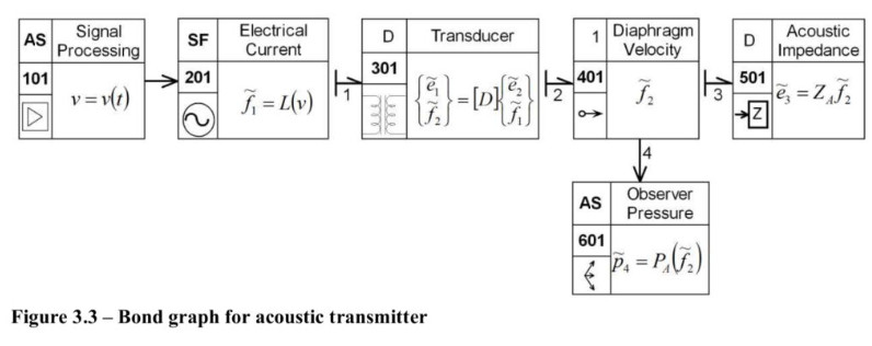
Figure 3.4 shows a high-level bond graph for the acoustic receiver system shown in Figure 3.1.
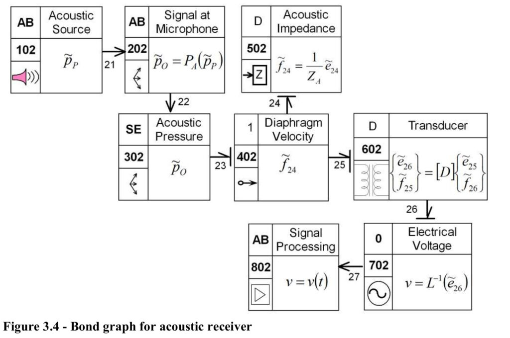
Note that Figures 3.3 and 3.4 introduce some symbols not previously mentioned. A full arrow indicates that a signal is sent from one element to another. Signals provide only information, not power. AB, AS, and D are element types used to indicate high-level elements that with the physics not yet fully defined.
The objectives of this chapter are development of methods for determining the acoustic impedance, ZA in elements D501 and D502, and the acoustic transfer function, between the transducer diaphragm velocity and the pressure at observation point, P. The transfer function is called PA in elements AS601 and AB202 in Figure 3.4. Several simple geometries will be considered. For more complicated situations, numerical methods or experimental measurements are necessary. Methods for characterizing transducer functions, D in elements D301 and D602, will be covered in the next chapter.
Figure 3.2 includes the separation distance, r, between the transducer and the observation point (or sound source and transducer in Figure 3.1). Thus the models are not 0-dimensional. The radiation signal models and the acoustic impedance models will depend in most cases on the geometry of the transducer and the separation distance compared to the wavelength of the acoustic waves. Thus it will be necessary to note the diaphragm size and range of r for which a particular model is valid.
Spherical Acoustic Waves
In Reference [7] (page 169), the acoustic wave equation is derived by combining:
- Euler’s equation of motion,
- The equation of state,
- The equation of continuity
to give

Variable p is the acoustic pressure, c is the speed of sound, and t is time.
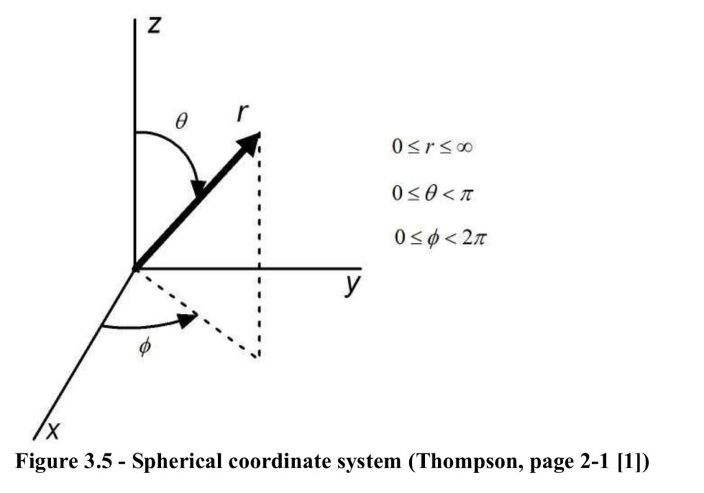
In spherical coordinates, shown in Figure 3.5
When the pressure field is independent of θ and ϕ, the wave equation simplifies to the axi-symmetric case

For harmonic steady state time dependence
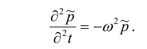
The tilde is used to indicate spatial amplitude. Equation {3.3} becomes the reduced wave equation (also called the Helmholtz equation):

Since time is not explicitly stated in {3.4}, it is normal practice to use wave number, k, rather than frequency, where

λ is the wavelength in meters, and f is the frequency in hertz.
Figure 3.6 shows the relationship between wave number and frequency for air with ca = 343 [m/s].
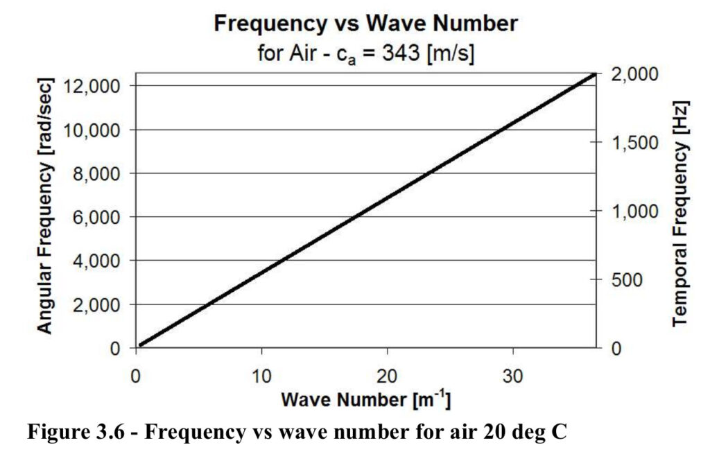
Extending the line in Figure 3.6 to 20,000 Hz shows that for sonic waves in air the wave number is between approximately 0.4 and 360 m-1.
The solution of {3.4} is the spatial amplitude of the pressure at any point at distance r from the origin

When the harmonic time dependence that was dropped from {3.3} is defined as
then the first term in {3.5} represents an out-going wave, and the second term represents an in-coming term. This can be seen by considering that a point on an out-going wave has

where C is a parameter for each point on the wave. Using this relationship, the location of any point r as a function of time is:

Equation {3.8} indicates that as time increases, r increases, which is the definition for an out-going wave. Some authors define the time dependence as
that reverses the meaning of the terms in {3.6}.
For a source in a free field, there are only out-going waves, so {3.6} reduces to

Since dynamic models use power variables, not only is the effort variable as a function of time needed, but also the flow variable. Equation {3.9} gives a relationship for pressure spatial amplitude, the effort variable. Corresponding to the effort variable,
is the flow variable – spatial particle velocity amplitude,
Analogous to Newton’s law relating force, mass and translational velocity, the acoustic equation of motion (Euler’s equation) relates pressure and velocity in a medium with density ρ0 ,

Substituting {3.9} into {3.10} gives an expression for the velocity amplitude from a spherical source:

Equation {3.9} indicates that the last factor in {3.11} is the pressure, thus

Equation {3.12} shows that for a spherical wave with constant pressure amplitude the velocity amplitude changes with distance from the source. This is in contrast to the relationship for a plane wave

where the velocity and pressure amplitudes do not depend on distance from the source.
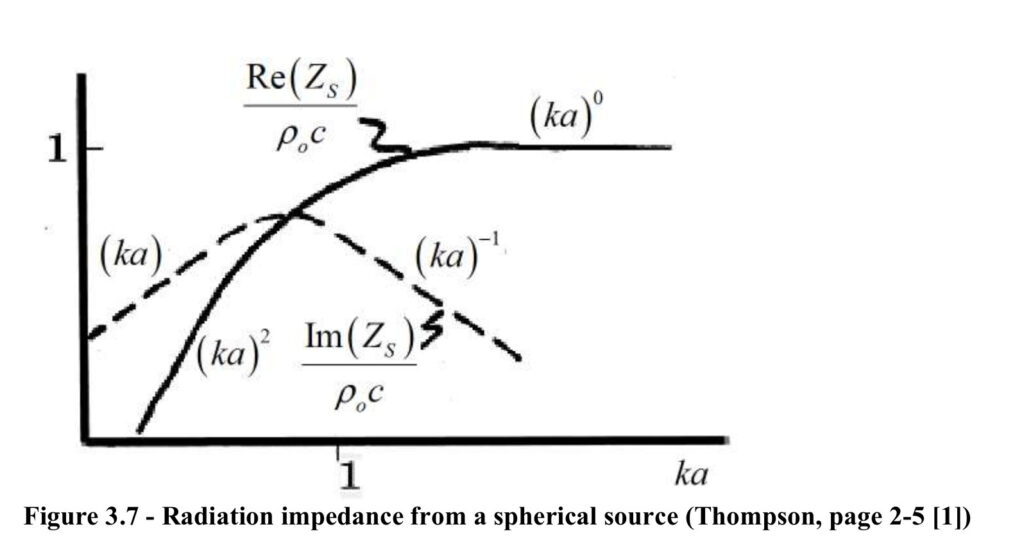
The ratio of the pressure amplitude and the velocity amplitude is the specific acoustic impedance, ZS. The subscript S indicates a spherical source. Equation {3.12} gives

The real and imaginary terms of {3.14} are separated to give the resistance and the reactance terms

Equation {3.15} shows that the pressure phase leads the velocity phase by angle Ψ where

As kr varies from 0 to ∞, Ψ varies from 90O to 0O.
For large kr, as r increases the spherical wave behaves more and more like a plane wave, i.e. ZS approaches ρ₀c.
Define
Re(ZS) = specific acoustic resistance
Im(ZS) = specific acoustic reactance.
Figure 3.7 conceptually shows how Re(ZS), Im(ZS) vary with ka, where a is the radius of the source. For small ka, reactance has the characteristic shape of a mass element, and the resistance for large ka is a constant.
Intensity
Pressure is a scalar quantity. Particle velocity is a vector. The product of pressure and particle velocity, called intensity, is a vector related to power. The average intensity, I, is the time average rate that energy flows through a unit area of the medium. Its units are [watts/m2].

The asterisk, *, indicates that the complex conjugate of
is
multiplied by
T is the period.
Substituting {3.12} into {3.17} and using
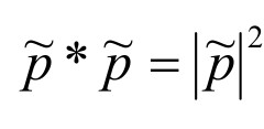
gives

Simplifying {3.18} gives

For the axi-symmetric case discussed here, I is independent of θ and ϕ, and since the surface area of a sphere of radius r is πr²,

For an energy conservative medium with
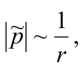
power, W, is independent of r.
For the general case, the pressure is a function of r, ρ and ϕ but in the far field (kr>16) Equation {3.19} still holds, and with the outward normal,
on surface S,

The following development will lead to equations for radiation from a speaker. This will be done by considering the simplest case of a monopole source, then expanding that to bipoles, dipoles, a hemispherical sources, and finally circular pistons which are good approximations to speaker cones. Similar development for symmetric arrays of point sources, and line sources can be found in Reference [1].
Monopole Source
A monopole, also called a simple source, is a pulsating sphere of radius a whose surface moves radially with uniform velocity. With the sphere located at the origin

Suppressing the harmonic time dependence

Assuming only outgoing waves (free field) Equations {3.9} and {3.14} give

Substituting {3.24} into {3.23} gives

Substituting {3.15} into {3.25}, solving for A, and replacing


Although {3.26} holds for all values of ka, of interest are the cases where the pulsating sphere is small compared to the wavelength, described by

With restriction {3.27}, {3.26} becomes

Source Strength
The source strength, QS, of a simple source is given by

So

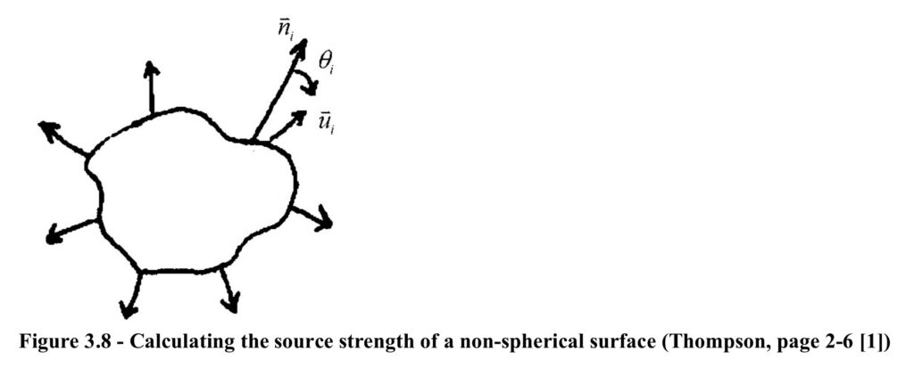
For a non-spherical source {3.30} holds if QS is calculated using

The factor
is the direction cosine of
each face of a pulsating polygon,
and
is the normal vector at each point on surface S.
Equation {3.31} says that the strength of any source is equal to the volume flow normal to the surface of that source as shown in Figure 3.8.
If a source is small compared to the shortest wavelength it emits, the radiated pressure is independent of the shape of the source. This characteristic makes differently shaped transducers have the same radiation impedance if their vibrating surfaces are small compared to wavelength.
In terms of source strength intensity, for a monopole, IM, and power, WM, are:


Directional Response of arrays of simple sources
In the last section, the radiation from a simple source was discussed. Now consider two in-phase simple sources separated by distance d as shown in Figure 3.9.
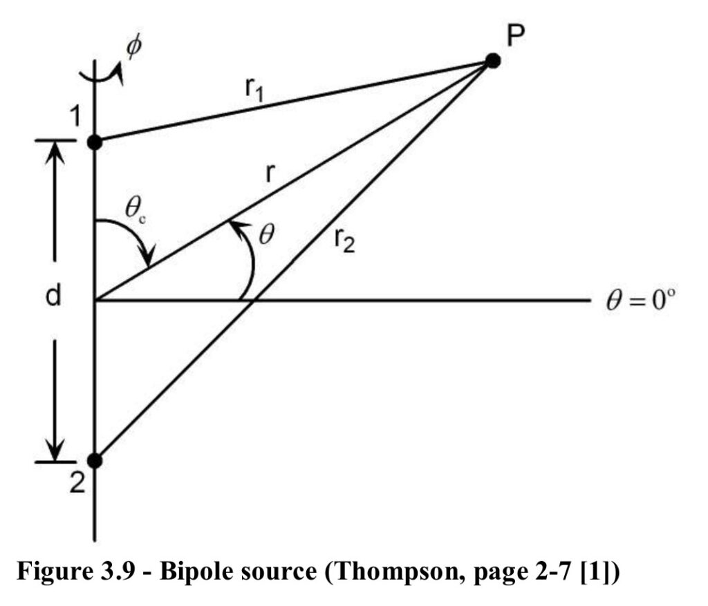
Using {3.30} the total pressure at P is the sum of the pressure from each source

With QS1=QS2=QS and


If point P is far from the sources, then referring to Figure 3.10, the distances r1 and r2 in the phase factors can be approximated by:

For the amplitude factors, further approximations are valid

The extra terms for the distances in the phase factors are needed because it is the wavelength difference between r1 and r2 that is important. For the amplitude factors, {3.38} can be used because it is the absolute magnitudes of r1 and r2 that are important. Therefore, {3.36} becomes


Applying the identities between trigonometric functions and complex exponential functions,


From Figure 3.9, the complement angle is
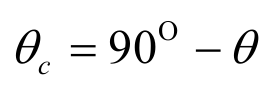
Therefore {3.41}could have been written as

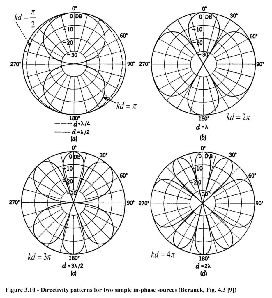
Equations {3.41} and {3.42} show that the pressure amplitude for a bipole depends not only on the distance r, but also the angular position of the point P with respect to the θ=0 plane. The term in square brackets in {3.41} (or equivalently in {3.42}) is an example of a directivity function, Γ(θ).
The absolute value of the directivity function

is a maximum at θ=0 or whenever
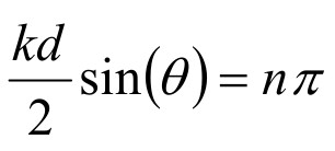
and the directivity function returns a value of 0 when

for all integer values of n.
Figure 3.10 shows plots of {3.42} for 4 alternative values of non-dimensional size parameter kd.
Dipoles
The bipole source in Figure 3.9 contained two simple sources pulsating in-phase. If the two sources are vibrating 180O out-of-phase, the array is called a dipole. When point P is far from the dipole the pressure amplitude is

Applying the identities {3.41} to {3.45} gives

or

Thus the directivity function for the dipole is

Equation {3.48} equals 0 at θ=0 and whenever

When
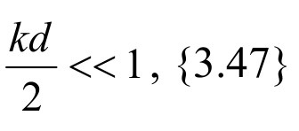
Equation {3.47} reduces to

The directivity function,
is a figure 8 pattern
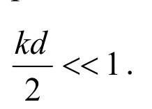
independent of frequency. Usually when someone speaks of an acoustic dipole it means that they are only considering the cases for which
The intensity for a dipole, ID, is

and the dipole power, WD is:

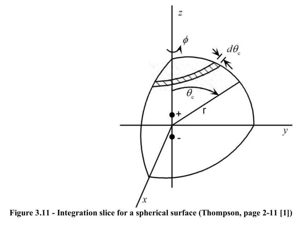
For a spherical surface with no ϕ variation, Figure 3.11 shows

then

Dividing {3.54} by {3.33} gives the ratio of the dipole power to the power of a monopole

Equation {3.55} shows that a dipole is much less efficient than a simple source.
Four In-Phase Point Sources with Uniform Spacing
The analysis of bipoles above can be extended to an array of 4 uniformly symmetric strength spaced in-phase simple sources shown in Figure 3.12.
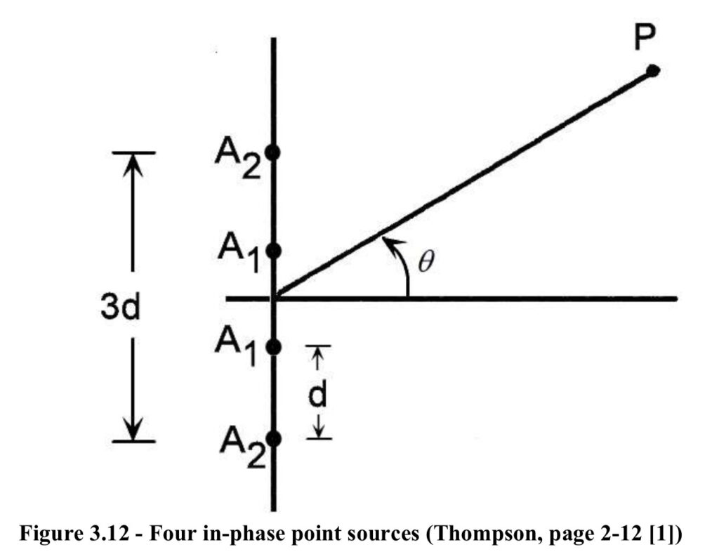
Symmetric strength means A1 and A2 do not need to be equal. The array can be considered a bipole with separation d, superimposed with a bipole with separation 3d. Then applying the results of Equation {3.41} gives


with

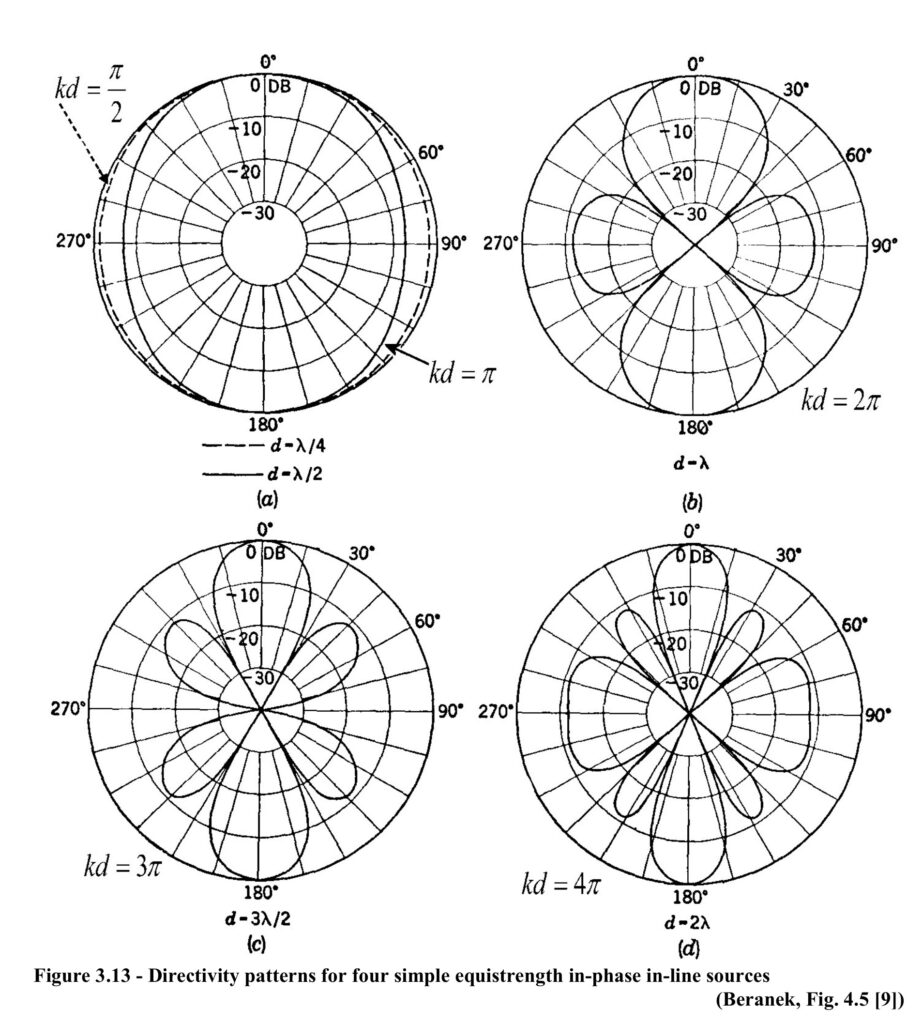
The directivity pattern for the array shown in Figure 3.12 for various values of kd is shown in Figure 3.13.
Hemispherical Source Mounted in Infinite Plane Rigid Baffle
The next steppingstone toward practical geometries is to consider the radiation pattern from a hemispherical source mounted in an infinite plane rigid baffle as shown in Figure 3.14. Figure 3.14 shows the equivalence of the radiation from a hemisphere in in an infinite plane rigid baffle to the radiation from a simple source.
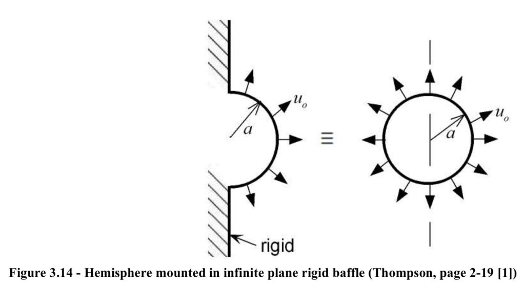
In Reference [7] Kinsler and Frey explain that when ka<<1, the rigid baffle imposes a boundary condition on the acoustic field in the right half plane such that

As with {3.29} the source strength is given by

But now the area is just that of a hemisphere of radius a, so

Therefore {3.58} in terms of source strength is

Comparing {3.61} with {3.30} shows that for QH= QS. The pressure produced by a baffled small source (small compared to wavelength) is twice as great as that produced by an unbaffled simple source.
As mentioned in Equation {3.32}, intensity is proportional to the pressure squared. Therefore, the intensity of a baffled small source is 4 times that of a simple source with QH = QS

Likewise, power for a baffled hemisphere is given by:

Radiation from a Plane Piston in an Infinite Plane Baffle
Figure 3.15 shows an arbitrary shaped plane piston (in the x-y plane)
vibrating with velocity
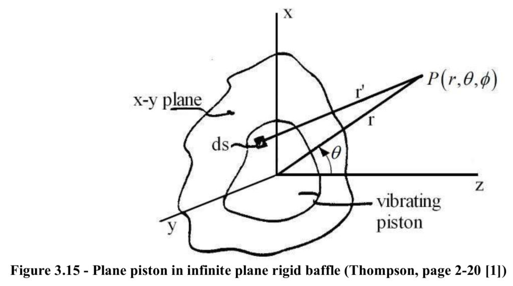
The source strength of patch dS is
{3.64}
where
is a unit vector in the z-direction.
At point P, the increment of pressure,
due to the
source at dS is

where r’ is the distance from dS to point P. Recall r is the distance from the origin to point P. To get the total pressure at point P, integrate the contributions from all the patches that make up the piston face. For an arbitrary piston shape, and non-uniform piston velocity such integration is normally done numerically.
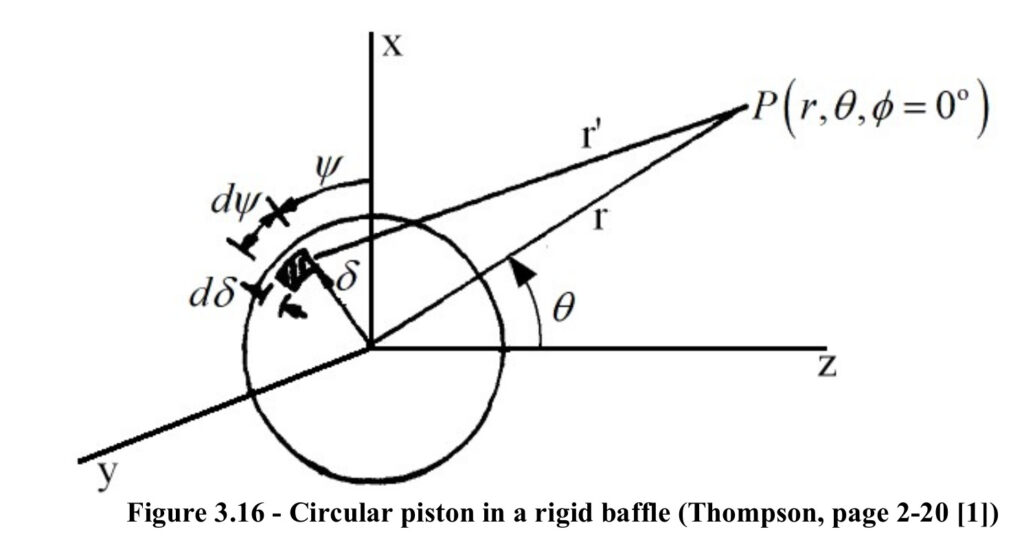
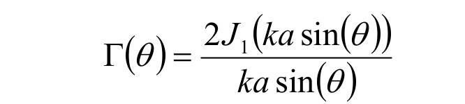
For a circular piston with uniform normal velocity amplitude, uO, as shown in Figure 3.16, the closed form has been found to include a directivity function in terms of a Bessel Function [7]

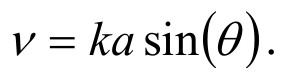
Figure 3.17 shows the value of the directivity function

where
A table of values for this function
can be found in [7].
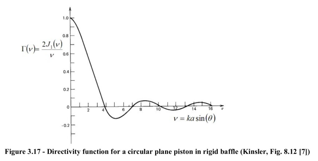
Figure 3.18 shows a beam pattern for a vibrating circular piston in an infinite plane rigid baffle with kd = 40.
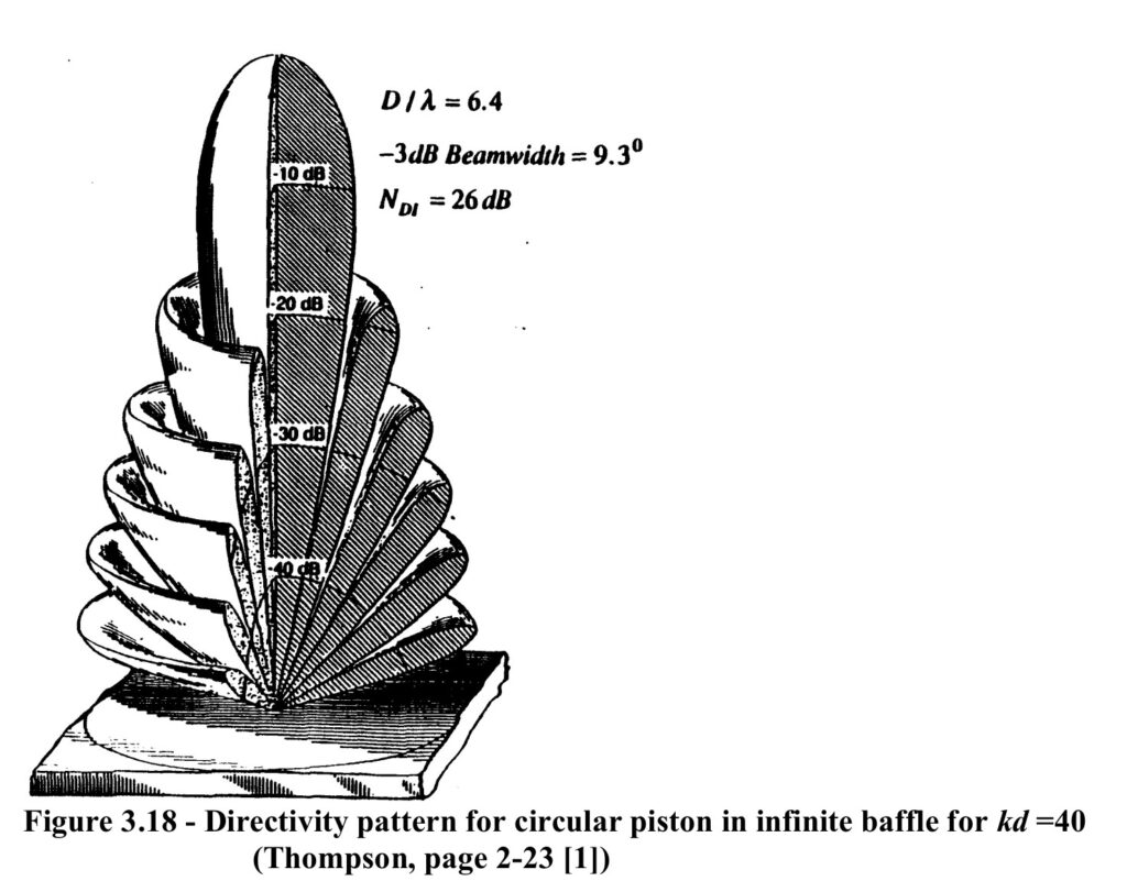
One use of the directivity function is to determine the beam width of either the sound pattern generated by a transmitter, or the sensitivity of a receiver. One metric for beam width is the -3dB level. This level occurs when
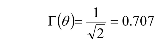
Interpolating the table in Reference [7] page 453 gives a value of

Therefore

then

Directivity Factor
Another metric used to describe directivity is the directivity factor ,γ. The value of the directivity factor varies with frequency. There appears to be various definitions for γ. Conceptually they are similar, referring to either the power or intensity produced by a source compared to either the power or intensity produced by a source compared to the same quantity generated by a point source. Here the definition used by Beranek [9] page 109.
Directivity factor is the ratio of the intensity on a designated axis of a sound radiator, at a stated distance r to the intensity that would be produced at that same position by a point source radiating the same total acoustic power. Free space is assumed for measurements. Usually the designated axis is taken as the axis of maximum radiation.
As indicated previously, power, W, radiated by a source is the integral of the intensity over an enclosing surface. For a sphere the average intensity is related to the power by:

with


Therefore

For the case with γ independent of ϕ

The direction of maximum radiation is called the principal axis. The directivity factor for the principal axis is therefore based on

Then {3.71} becomes

From {3.67}, for a circular piston in an infinite baffle the Normalized Directivity Function is:
Thus {3.71} and {3.72} gives

For ka<<1
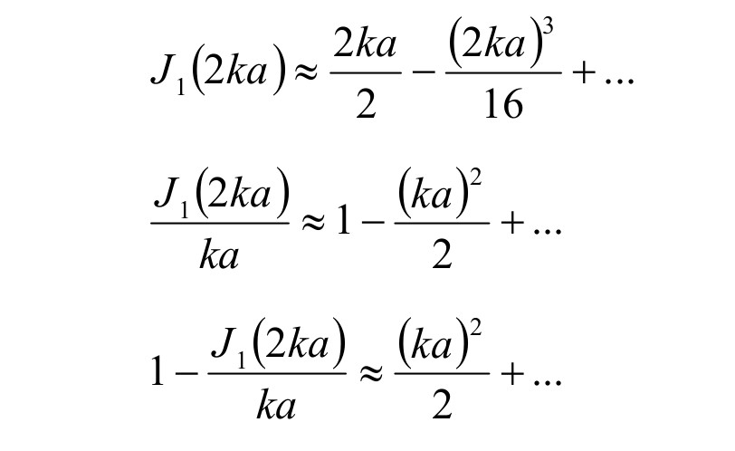
therefore

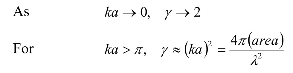
For large ka:
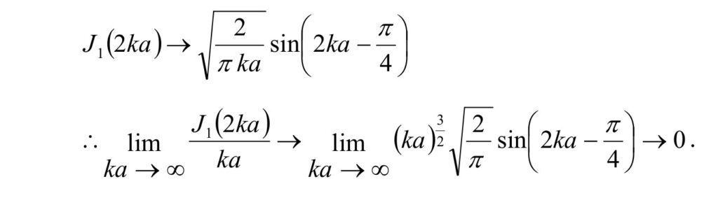
Therefore for large ka

where S is the area of the piston. Equation {3.77} is valid for any shape plane piston radiator of area S with uniform velocity provided its dimensions are greater than a wavelength.
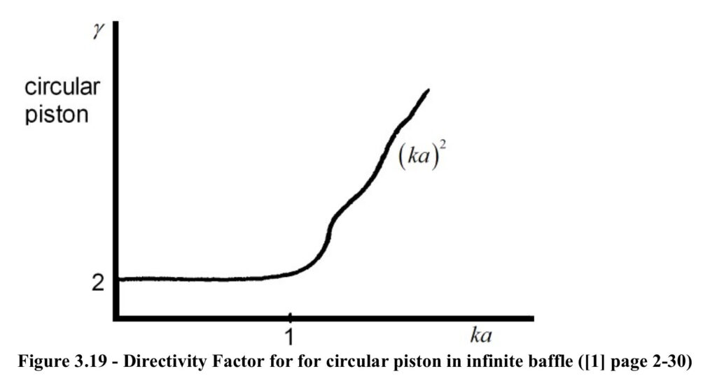
Figure 3.19 is a plot of {3.75} showing the low frequency part given by {3.76} and the high frequency part given by {3.77}.
When a piston does not have uniform velocity but rather has more motion in the center than at the edges, the condition is called amplitude shading.
Amplitude shading causes:
- Reduced side lobes which increases γ
- Broadens main lobes which decreases γ
- Net result is usually a decrease in γ
Directivity Factors of Various Sources
For reference, the directivity factors for several common sources are given in this section. These directivity factors are determined using the relationships in {3.74} and the directivity functions for each case.
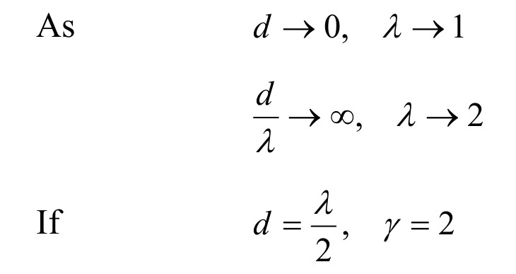
2 equistrength, in-phase point sources
Using the directivity function {3.44} gives

Uniform velocity circular piston source
With piston radius, a

Uniform velocity rectangular source
When both dimensions h and w are greater than wavelength,
{3.80}
Uniform velocity piston of any shape
When all dimensions are greater than wavelength,

Pressure Field on the Axis of a Circular Piston Source
A common parameter of interest is the far field pressure amplitude on the axis of the transducer face. Often the source can be considered a circular piston. Along the normal axis of the piston as shown in Figure 3.20, the distance to any point on the axis to any point on the piston is r’

and the pressure amplitude on the axis due to a small patch on the piston is

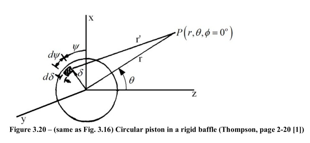
Integrating the patch over a ring of the surface yields a factor of 2π and then integrating along the radius of the piston gives

Using substitution of variables let

therefore

gives

By factoring out the average value for the exponent of the exponential

then transforming the complex exponentials in the brackets to the sine function

gives

Since the sine square varies from 0 to 1, the normalized pressure
amplitude squared on axis,
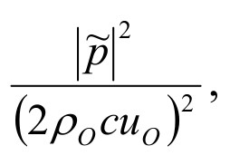
varies between 0 and 1
as shown in Figure 3.21 for some arbitrary value of ka.
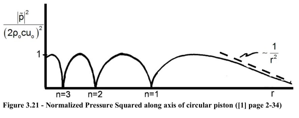
The zeros in Figure 3.21 occur whenever

or
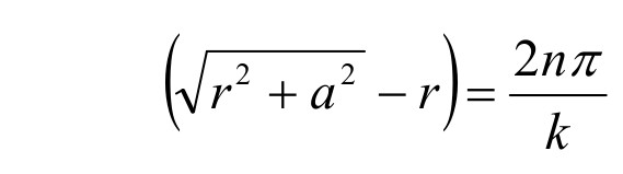

The largest value of r for which a zero occurs corresponds to n=1

If a is <λ, a positive value of r is not possible.
The largest value of r for which a maximum can occur is when

Unless 2a >λ, a positive value for r is not possible. If 2a is much greater than λ, the last term in {3.93} is small giving

If r is even bigger, say
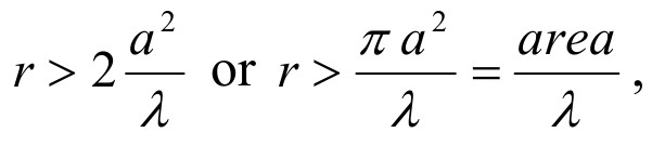
there is spherical
divergence of the sound field, i.e.
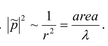
This relastionship
can be seen by considering equation {3.89} for large r,

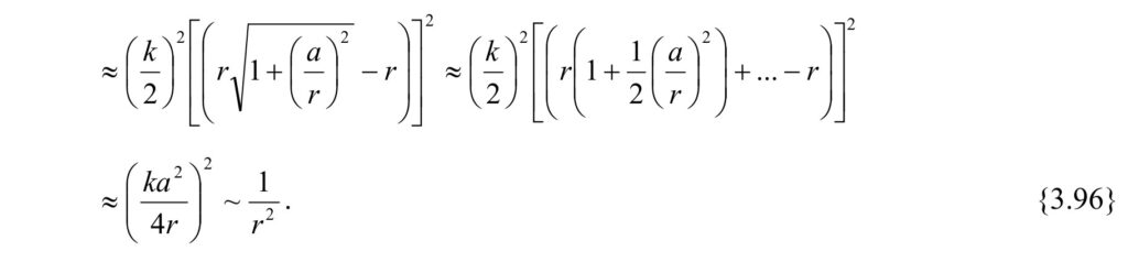
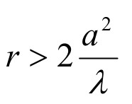
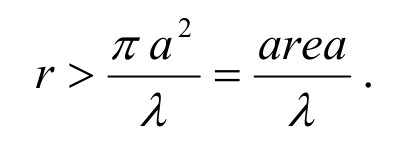
This relationship is the rationale for the rule of thumb when calibrating a transducer that requires a minimum separation distance between the
source and receiver of
or
Radiation Impedance Load on Uniformly Vibrating Circular Piston
One of the most useful relationships when analyzing the frequency response of a transducer is the force the medium imposes on the radiating face for a given velocity. The relationship (force/velocity) is called the radiation impedance.
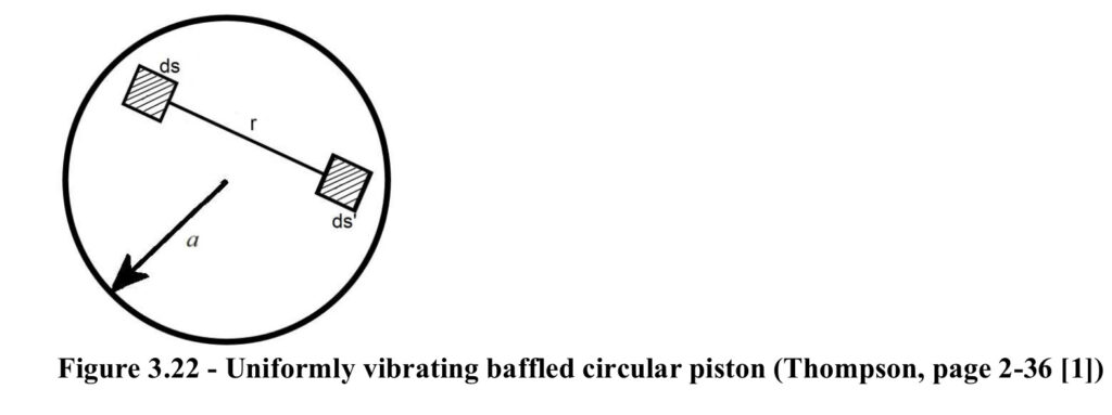
Consider the circular baffled piston shown in Figure 3.22, with radius a, and constant normal velocity amplitude uO.
As before, the pressure amplitude at any point due to the motion of a small patch dS is

The location of interest is not now at an arbitrary point in space, but rather another patch on the surface of the piston noted as dS’ in Figure 3.22. By integrating over the surface of the piston the total pressure is determined at each point on the piston to give

Equation {3.98} shows that the pressure amplitude varies with position even for constant velocity amplitude.
The total acoustic force amplitude on the piston is determined by integrating the pressure for each point on the piston


Equation {3.100} is valid for any shape plane piston and even for disjoint areas, as long as the face velocity is uniform. Numerical integration is required to solve {3.100} for most cases, but the integration can be done analytically for a circular piston.
The mechanical radiation impedance, ZR, is defined as the acoustic force amplitude, Eacoustic, divided by the velocity amplitude, uo. This complex impedance can be separated into the real terms, radiation resistance, RR, and the imaginary terms, radiation reactance, XR.

The piston resistance function, R, and the piston reactance function, X, is obtained by factoring out a constant to give

For a baffled circular piston the resistance function, R, is

where J1 is the Bessel Function of the first kind of order 1. The reactance function, X, is

where H1 is the Struve function of the first kind of order 1.
The Struve function with argument, z, is determined from the series

For small ka:

and

For large ka:

and

Figure 3.23 compares the normalized radiation impedance of a sphere to a circular piston. The general shapes of both the resistance and reactance functions are similar. The circular piston resistance curve above ka = 1 display ripples characteristic of a Bessel function. The reactance curve above ka = 1 has ripples because of the Struve function in its defining equation.
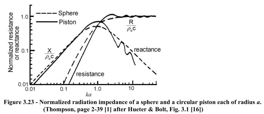
Reference [1] shows similar plots for pistons with other geometries.
Accession to Inertia
The radiation reactance, X, of a single isolated radiator is always positive indicating that it is a mass-like impedance. At low frequencies, X varies with ω. For example{3.107} gives

therefore

Meq is called the accession to inertia. Imagine Meq to be a mass of fluid of cross sectional area
and height
then

Solving for

The factor 0.85a is called an end correction – the apparent length is that of the equivalent mass. The mass reactance effect always lowers the resonance frequency of a vibrating transducer or structure.
Radiated Acoustic Power
The effective acoustic resistance for a uniformly vibrating piston is related to the radiated acoustic power, W by:

For low frequencies (small ka)

where

therefore

As stated in Equation {3.59} the source strength QH is defined as the product of area, S, and velocity amplitude, uO. Thus {3.117} can be written as

Low frequency RA is independent of geometry, but QH changes with source size.
For high frequency

giving

With all the preliminary work completed, the following chapter will focus on the ideal behavior of electro-acoustic audio transducers.